Category Archives: Guest Weblogs

Guest Post – Climate Change Predictions, Including Extreme Hydrometeorological Events By Dr. Millán Millán

We are very appreciative to have a guest post by Millán Millán, Executive Director, Institute CEAM-UMH in Spain. With my encouragement, he has accepted posting his excellent presentation this past summer

GUEST POST

 European Union-United Nations International Strategy for Disaster Reduction

 EU-UNISDR International Workshop, Brussels, 6-7 July 2010. Reducing Water-Related Risks in Europe

 Climate Change Predictions, including Extreme Hydrometeorological Events.

by Dr. Millán Millán, Executive Director, Institute CEAM-UMH, Spain.

1.  Introduction:  A letter to Dr. Fritz Holzwarth, Director General for Water-Management, German Federal Ministry for the Environment, Nature Conservation and Nuclear Safety (12 July 2010).

Dear Dr. Holzwarth, enclosed please find a summary of our findings on the hydrological cycle in Southern Europe.

Data from European Projects from 1974 to the present have been re-analysed in the context of a perceived loss of summer storms around the Mediterranean (Millán et al. 2005a, b).  In this respect, the first point to emphasise is that, geographically, Europe lies within two separate Hydrological Basins.  That is, one part of Europe is in the North Atlantic Catchment Basin and the other part is in the Mediterranean Catchment Basin (Figure 1).  The two are separated by the European Continental Divide, as illustrated in Figures 1 and 2.  Our findings show that the hydrological cycle in these two parts operates differently.  In the European regions north and west of the Continental Divide, the Atlantic Catchment Basin gets most of its water from “Classic weather systems”, i.e., travelling depressions and their associated fronts coming from the Atlantic.  Land-use changes within this divide will mainly affect the capacity of the surface to retain water, and, thus, they can affect the frequency and intensity of floods.

In contrast, on the Mediterranean side of the European Divide, the Atlantic precipitation component is weak or non-existent (e.g., Greece, Turkey), and the main precipitation comes from summer storms and Mediterranean Cyclogenesis.  The latter events can be triggered either by orographic lift and/or by the advection of an upper perturbation (i.e., cold trough aloft) moving south from more northerly latitudes.  This has caused some meteorologists to classify Mediterranean Cyclogenesis events as resulting from “Atlantic fronts” when, in reality, the water vapour involved in the precipitation has mainly originated within the Mediterranean Basin (Pastor et al. 2001).  In other words, most of the water that precipitates in summer-storm and Mediterranean-Cyclogenesis events in the Mediterranean Basin has been evaporated from, and is thus recirculated within, the Mediterranean Catchment itself.  Having identified this, our findings further suggest that land use is a key component in this process as it governs both how much, and how, the water is recirculated in this basin.

Our study shows that summer storms around the Western Mediterranean Basin are directly affected by land-use changes, and when these storms are lost, a chain of events is triggered which leads to an accumulation of water vapour over the Mediterranean Sea and an increase in summer floods in Central Europe.  Moreover, the focuses for the most intense summer precipitation (and flood) events, involving Vb tracks, seem to occur right along the European Continental Divide (Figures 2, and 3), and could also result from the convergence of Atlantic and Mediterranean moist airmasses.

Another problem is the common assumption, with respect to the hydrological cycle, that the water resource is universally provided by precipitation from the large weather systems.  As this is not true in most parts of the world, the notion that the water resource is there and all that is required is to manage it properly is perhaps the most widely extended fallacy regarding the water cycle (in Europe).  In the northern hemisphere (Figure 1), this assumption holds only in the Atlantic and Pacific Divides north of » 35º North Latitude.  Moreover, it can only be truly asserted for the western (oceanic) sides of the continents, i.e., the European-Atlantic and American-Pacific sides of the continents.

For any other Water Catchment Basin in the world, other processes must be considered.  For example, the available precipitation in the Central North American Basin, which is lodged between the Pacific and North Atlantic Divides, is strongly modulated by conditions in the Gulf of Mexico, i.e., by processes and conditions at the Regional to Subcontinental scales.  In tropical forest areas (i.e., rainforests), after a massive inflow of water vapour at the beginning of the wet season, the water is basically recirculated between the soil-forest and the atmosphere, producing a daily afternoon-evening shower.  Thus, rainforest means exactly that: take the forest away and the rain goes along with it, allowing the area to become a desert and/or prone to major floods.  The rainforest is probably the ultimate case in which surface properties govern the precipitation during the wet period.

A synthesis of our findings on the hydrological cycle in Southern Europe and its possible consequences for the rest of the continent is presented in Figure 4 (EC 2007).  This is discussed in more detail in a report prepared for Peter Gammeltoft (DG ENV) from work done within the EC CIRCE Integrated Project, i.e., the Gammeltoft-CIRCE_RACCM report.   Some of the details, and the implications for Climate Models, were discussed at the EC_UNISDR Workshop,  Brussels 6-7 July 2010, and the extended Abstract is included below.

2.  Extended Abstract  EU-UNISDR International Workshop, Brussels, 6-7 July 2010.

“It is very likely that hot extremes, heat waves and heavy precipitation events will continue to become more frequent”.  This is a conclusion common to all IPCC Assessment Reports.  However, “although the ability of Atmosphere-Ocean General Circulation Models (AOGCMs) to simulate extreme events, especially hot and cold spells, has improved, the frequency and amount of precipitation falling in intense events are underestimated” (IPCC 2007).  It is also likely that the latter situation will continue for a long time, that is, unless the meteorological basis of current Climate Models manages to become able to simulate specific local-to-regional processes, such as land-atmospheric-oceanic feedbacks or the folding of boundary layers in complex coastal terrains in the sub-tropical latitudes.

Nevertheless, some of the observed anomalies and results of these processes were indeed addressed both in the Fourth Assessment Report AR4 (IPCC 2007) and in the earlier Third Assessment Report TAR (IPCC 2001), as information resulting from EC research filtered into the system. In this context, the present work reviews some of the processes that should be considered to improve AOGCMs, with reference to specific quotes and comments in the AR4.

Information gathered during various European Commission (EC) research projects in the areas of Atmospheric Chemistry and Desertification, i.e., some 37 projects from 1974 to 1994, had alerted of a loss of summer storms around the Western Mediterranean Basin.  This issue was addressed in 1995 by re-analysing the meso-meteorological information obtained in nine of the EC projects and disaggregating the precipitation components for one of the experimental areas used in these projects (Valencia, eastern Spain).  The results of the analysis (Millán et al. 2005a, b), shown in Figure 5, identify three sources of rain in this region, viz: Atlantic Fronts which contribute <20% of total precipitation; Summer Storms, 11% to 16% of total precipitation; and Mediterranean Cyclogenesis, >65% of total precipitation.  These precipitation components come from different weather patterns.  Moreover, the correlation of the Atlantic fronts with the NAO (North Atlantic Oscillation) is negative while the correlation with Mediterranean Cyclogenesis is positive (Millán et al 2005b).

This situation regarding the origin of the precipitation components appears to be the norm, rather than the exception, in the entire Mediterranean Basin and probably in other subtropical areas of the world, which include a very important part of the Global Climate System.  Furthermore, in the Mediterranean Basin the contribution from Atlantic depressions has been decreasing for the last 50 years, summer storms over the mountains surrounding the Mediterranean Sea have nearly disappeared in the last 30 years, while extreme precipitation events associated with Mediterranean Cyclogenesis appear to be increasing rapidly and becoming more torrential in nature.  It is important to emphasise this because current Coupled AOGC Models are unable to distinguish between precipitation components in these latitudes. Finally, our analysis of EC project results shows that both summer storms and intense precipitation events due to Mediterranean Cyclogenesis appear to be governed by land-use-atmospheric-oceanic feedbacks.

For example, summer storms form (or used to form) in the afternoon over the mountains surrounding the western Mediterranean basin at 60 to 80(+) km from the sea, as the final stage in a coastal wind system that develops during the daytime in summer and combines the sea breeze and the up-slope winds, henceforth called the combined breeze.  The specific characteristics of this wind system have been documented in several European Commission projects (Millan et al. 1997; 2000, 2002) and derive from the nature of the Western Mediterranean Basin (WMB).  That is, a large and deep sea, totally surrounded by high mountains in the subtropical latitudes. The following features make this wind system different from a “classic seabreeze” (Munn 1966, Stull 1988):

(1)  Upslope wind cells develop early in the morning, i.e., right after sunrise, over the east-and-south facing slopes (Millán et al. 1991,; 1992). 

(2)  The seabreeze develops at mid morning and, during July-August, its average duration and the wind travelled distance at the coast are, respectively, 14 hours and 160 km (Millán et al. 2000).

(3)  The seabreeze progresses inland in a stepwise manner, by incorporating one after another the up-slope wind cells formed earlier that day (Figure 6).  This is in contrast to the smoother penetration in a classic seabreeze over flat coastal areas. 

(4)  After advancing each step, the leading edge (or front) of the combined breeze can remain stationary over that position for » 1/2 to 1 hour, or more.  This process was first observed after tracking the evolution of the small cumulus clouds forming at the leading edge of the breeze (Millán et al. 1992)

(5)  It can take from » 4 to 6 (+) hours for the front of the combined breeze to reach all the way from the coast to the top of the mountains 60 to 100 km inland.

(6)   Once the front reaches the mountain tops, it tends to become locked onto that position, i.e., this becomes the last step, and it remains there for 4 to 6 h, until the end of the breeze period (Salvador et al. 1997).  

At the leading edge of a “classic” seabreeze a curtain of air is uplifted from the surface and injected into the return flows aloft, while the seabreeze front progresses smoothly inland (Munn 1966).  In the combined breeze, however, the front advances to a certain position and remains there for a period of time, until the breeze front moves (jumps) to the next position, and so on.  Because the positions of the front are conditioned by the orography, and the injection over each of those points resembles the mechanism creating “chimney clouds” (Huschke 1986), the term convective-orographic “chimney” will be used henceforth to describe the situation described.  Thus, during the stationary period, a considerable part of the airmass reaching the front from the surface becomes injected directly into the return flows aloft, and the length of the layers formed at each chimney (see below) could be comparable to the distance that separates the base of that chimney from the previous one.

Another noteworthy feature is that the altitude of the injections increases at each new position of the leading edge, i.e., at each newly formed chimney, both because the airmass gains potential temperature as it follows a longer path along the heated surface, and because the base of consecutive chimneys occurs at ever increasing heights up the mountain slopes.  Finally, at each step, the return flows move seaward and sink (subside) along their way.  The amount of sinking that the return flows sustain is also comparable to the altitude of the base of the chimney in which they were injected.  Finally, the sinking also tends to increase the stability of the returning airmass and favours the formation of layers over the coastal areas and the sea (Figure 7, Millán et al. 2000).  All of these mechanisms form part of a “closed” vertical circulation loop that grows during the day, reaches its maximum development in the afternoon, and ceases by evening, only to begin anew the following day.

The number of steps that the combined breeze takes to reach the mountain ridges inland and, thus, the number of chimneys and layers formed during its development depend on the lay of the slopes around the Western Mediterranean basin (Figures 7, 8 and 9).  During this process, storms can develop whenever the Convective Condensation Level (CCL) of the incoming air mass is reached within the leading edge of the combined breeze, i.e., at its current chimney position.  This can trigger deeper (moist) convection and the development of a storm.  Finally, if storms do develop, the air mass becomes mixed all the way up to the tropopause, and the closed-loop coastal wind system becomes “OPEN”.  That is, the described wind system ends up behaving like a small monsoon.

The formation of storms, however, requires the addition of water (e.g., evaporated from the surface, wetlands, irrigated crops, etc.) to the airmass coming inland from the sea.  This is required to counterbalance the heating that the air mass sustains as it moves inland along the heated surface, and bring the CCL of the incoming airmass below its height of injection into the return flows aloft.  Otherwise, heating prevails and the CCL of the incoming airmass will keep on rising, the combined breeze will keep progressing inland, and a “first critical threshold” (or tipping point) in this wind system will be crossed when the CCL becomes higher than the height of the injections over the mountain tops.  Under these conditions the coastal circulations will stay “CLOSED”.  That is, storms will not develop, and the return flows aloft will continue moving seaward during the entire day, forming layers that contain the non-precipitated water vapour and the pollutants carried by the combined breeze, and piling them up to 4500(+) m over the Western Mediterranean Basin (Figure 8).  Moreover, because summer precipitation will decrease if storms do not develop, the conditions that maintain the combined breeze as a “closed” wind system (viz. insufficient evaporation along its surface path) can be considered part of a first feedback loop that tips the local climate towards increased drought inland (Figure 4). 

To simulate these processes, e.g., the development of the sea breeze, mesoscale meteorological models require the use of grids smaller than 10 km x 10 km (Salvador et al. 1999).  But even when using smaller grids (i.e., 5 km x 5 km) and vertical resolutions at the limit of numerical instability (e.g., 36 m), current models are not able to reproduce all the structures documented experimentally over the Western Mediterranean (Figure 9).  This can be considered relevant as AR4 Section 8.2.2.2 Horizontal and Vertical Resolution states that “Changes around continental margins are very important for regional climate change”.

Moreover, if these closed-loop conditions develop in other coastal areas of the Western Mediterranean, they can become self-organised during the day to originate a meso-a scale circulation extending to the whole Basin.  In this case, the chimneys at the leading edges of the combined breezes will join together to form well-defined convergence lines along the mountains surrounding the basin, i.e., some 60 to 100 km inland from the coasts  (Figure 10).  As a result, a generalised and intense compensatory subsidence will also develop over the coastal areas and the sea which will keep the surface layer confined below ≈ 200 m (Figure 11).  This vertical confinement has been observed to extend all the way from the coast to each of the orographic chimneys formed along the path of the combined breeze and, eventually, to the last chimney that forms in the late afternoon as far as 80 to 100 km inland.  These boundary layer depth values, and typical rates of evaporation over irrigated areas and mountain maquia, were used to estimate the critical thresholds illustrated in Figure 9.

In the Western Mediterranean Basin, the “closed loop” conditions have been documented to last from 3 to 9 consecutive days, and recur several times a month, i.e., for a total of 12 to 24 (+) days per month, from late spring to late summer (May-September).  During these periods the Western Mediterranean Basin behaves like a large cauldron that boils from the edges towards the centre.  In this cauldron, each day, the coastal circulations recirculate (vertically) from » 1/4 to 1/2 of the depth of the layers accumulated over the sea on the previous days.

The self-organisation of the local circulations from the meso-g scale (to » 20 km), through the meso-b scale (to » 200 km), to a full-fledged meso-a scale (to » 2000 km) circulation during the day can be considered a good example of atmospheric properties and processes spilling up and down the meteorological scales, typical of sub-tropical latitudes.  It also means that when storms do not develop, at each step in the penetration of the combined breeze, part of the air travelling along the surface becomes injected into the return flows and folds over the top of the return layers formed in the previous step (Figures 7 and 8).  Therefore, the temperature and humidity profiles observed over the coastal areas and the sea are the result of the systematic folding of the surface boundary layers over the sea on several consecutive days, together with other processes, e.g., the sinking and re-stacking of the layers according to their potential temperatures, too complex to discuss here.

The development of large meso-scale circulations around large-enclosed (Mediterranean) or semi-enclosed (e.g., Sea of Japan) seas could underscore two other aspects mentioned in AR4 when referring to Continental edge effects and lapse rates (8.6.3.1 Water Vapour and Lapse Rate).  This document states that “In the planetary boundary layer, humidity is controlled by strong coupling with the surface, and a broad-scale quasi-unchanged RH response is uncontroversial”.  The uncontroversial part of this statement could be just another fallacy regarding the Atmosphere-Land connection in Climate Change Models (Figure 13).  That is, for any region outside flat terrains in mid latitudes.  The statement is false because when the edges of the continents wrap around a large interior sea like the Mediterranean, or a large semi-enclosed sea like the Sea of Japan, Continental Edge effects blend together to create their own large meso-meteorological circulation and dominate the weather patterns in these regions for months.

Finally, the “Continental Edge Effect” becomes particularly important if the continental edges are backed by complex coastal terrains, that is, coasts backed by high mountains up to 80(+) km from the sea.  The reason for this, as related above, is that the combined breezes make the coastal boundary layers fold over themselves, creating a multitude of “residual boundary layers” piled-up several km high over the enclosed seas.  The EC’s MECAPIP and RECAPMA (MEso-meteorological Cycles of Air Pollution in the Iberian Peninsula – MECAPIP, 1988-1991, REgional Cycles of Air Pollution over the West-Central Mediterranean Area – RECAPMA 1990-1992) projects documented as many as 7 layers piled-up over the Mediterranean to 4500 m (Millán et al. 1992), which could explain the observed temperature lapse rates (Figures 7 and 8) and the water vapour profiles observed over some coastal areas, and over large interior seas in sub-tropical latitudes.

The observed profiles include temperature increases from 13K to 19K in the return flows (Figure 8) and a higher water content (i.e., perturbed RH) in the upper layers than in the layers directly above the sea.  This is the result of the evaporation added during their flow path over land (albeit not enough to trigger storms, as mentioned above).  The observed temperature and moisture profiles can thus be considered “anomalous” with respect to current advection-dominated model simulations, which assume that the water vapour is evaporated directly from the surface (or comes from upstream).  And because the models are unable to simulate the systematic folding of the surface boundary layer over itself for several consecutive days, they cannot simulate the resulting accumulation of atmospheric properties (i.e., temperature, pollutants and water vapour) in layers over the coastal areas and the (large interior) sea.

Current numerical simulation models, even when using 2km x 2km grids, do not capture all the details of the observed processes; e.g., they cannot reproduce either the vertical recirculations or the layering over the sea.  Nevertheless, the outcome of these processes, i.e., the development of an accumulation mode for water vapour (and pollutants) over the sea, has been validated with water column data from NASA-MODIS ever since the year 2000 (Figure 13).  MODIS data (Gao and Kaufman 2003) show that there is an intense and prolonged accumulation mode over the Western Basin and the Black Sea in summer, and two weaker accumulation modes over the Eastern Basin in spring and autumn.

These vertical recirculation-accumulation modes make the weather and climate in the Mediterranean Basin, and other semi-enclosed seas in the subtropical latitudes, very different from in the mid latitudes.  Thus, in contrast with regions dominated by advection, in the Western Mediterranean Basin, water vapour and pollutants can accumulate in layers piled-up to 4500(+) m over the sea, for extended periods during the summer.  And, without requiring the high evaporation rates of more tropical latitudes, the above-described mechanisms are able, in just a few days, to generate a very large, deep and polluted air mass that increases both in moisture content and in potential instability with each passing day.

The accumulation periods end (i.e., every few days) when the moist and polluted air masses are vented out of the area by an upper atmospheric perturbation.  Under certain conditions the accumulated water vapour can contribute to an increase in intense precipitation events and summer floods in Central and Eastern Europe.  Finally, during the vertical recirculation-accumulation periods, the greenhouse effect of the water vapour (Figure 14), photo-oxidants (ozone) and aerosols accumulated in layers over the sea enhances sea surface temperature heating during summer.  This propitiates a second feedback loop where Mediterranean Cyclogenesis fed by a warm(er) sea (Pastor et al. 2001) contributes to an increase in torrential rains and floods in Mediterranean coastal areas from autumn to spring (i.e., effects delayed by a few months with respect to the closing of the first loop).

In this second feedback loop another “critical threshold” may then be crossed if torrential rains, during intense Mediterranean Cyclogenesis events, trigger flash floods and/or mud flows over mountain slopes already affected by the first feedback loop, i.e., drier and vegetation-deprived.  This can increase erosion and/or produce massive soil losses which, in turn, can further reinforce the first feedback loop and help propagate its effects (desertification, drought), to other parts of the Mediterranean basin.  Available evidence indicates not only that these processes and feedbacks have been operating in the Mediterranean for a long time, but also that fundamental changes and long-term perturbations to the European water-cycle (extended droughts and intense floods) are taking place right now.

This analysis further suggests that: up to 75% (or more) of the precipitation in southern Europe, i.e., from Summer storms and Mediterranean Cyclogenesis, originates from water that first evaporates and then precipitates, i.e., it is recirculated, within the major Mediterranean drainage basin (i.e., all the areas south and east of the European Continental Divide including the Mediterranean and Black Seas).  Moreover, on the Mediterranean side of this Divide, rain of Atlantic origin contributes less than » 20% of the total (probably even less than that in Greece), whereas on the Atlantic side of the European Divide, » 80% to 90% or more of the precipitation is from water evaporated over the Atlantic Ocean.

Finally, land-use appears to play a key role in the loss of summer storms, the shift to more frequent vertical recirculation periods, and the amount of water recirculated within the Mediterranean basin.  These findings and the questions they raise are critical for the Mediterranean side of the European Divide:

 (a)    Drought and torrential rains in areas around enclosed seas in the subtropical latitudes (e.g. Mediterranean, Sea of Japan, South China Sea?) are the result of the same concatenated meteorological processes involving atmosphere-land-oceanic feedbacks.

(b)    The same processes can also lead to intense precipitation events and summer floods in other parts of Europe (i.e., points along the European Continental Divide, or within the  Mediterranean Catchment side of the Divide). 

(c)    Moreover, through the intensification of the Atlantic-Mediterranean Salinity Valve, the North Atlantic Oscillation could be perturbed and affect precipitation regimes on the Atlantic side of the European Continental Divide.

(d)    That is, the local-to-regional perturbations initiated by land-use changes at the local level can propagate their effects to the Global Climate System.

(e)    The basic atmosphere-land-ocean exchange governing these processes is not (and probably cannot be) included in current Atmosphere-Ocean General Circulation Models (AOGCMs).

(f)     Thus, the feedback processes in the hydrological cycle, which govern the partitioning and recirculating of water vapour and precipitation, as well as the development of extreme hydro-meteorological events, cannot currently be simulated in the AOGC Models used to assess extreme events in sub-tropical latitudes.

This situation now presents the research community with very important challenges to improve current Atmosphere-Land-Oceanic parametrisations in Atmosphere-Ocean General Circulation Models.  It confirms that hasty decisions on the future of the water cycle could be wrong and have catastrophic consequences not only for Southern Europe, but also for the rest of Europe. 

REFERENCES

European Commission, 2007: International Workshop on Climate Change Impacts on the Water Cycle, Resources and Quality. Report EUR 22422. Luxembourg: Office for Official Publications of the European Communities, 149. ISBN 92-79-03314-X

Gao B.-C., Y. J. Kaufman, 2003: Water vapour retrievals using Moderate Resolution Imaging Spectroradiometer (MODIS) near-infrared channels, J. Geophys. Res., 108, NO D13, ACH 4-1, 4-10.

Huschke, R.E. (Ed.), 1986: Glossary of Meteorology. American Meteorological Society, Boston, Mass., 638 pp.

IPCC, (TAR) 2001: Climate Change 2001: Synthesis Report. A contribution of Working Groups I, II, and III to the Third Assessment Report of the Intergovernmental Panel on Climate Change [Watson, R.T. and the Core Writing Team (eds.)].  Cambridge University Press, Cambridge, United Kindom, and New York, NY, USA, 398 pp.

IPCC, (AR4) 2007: Climate Change 2007: The Physical Science Basis. Contribution of Working Group I to the Fourth Assessment Report of the Intergovernmental Panel on Climate Change [Solomon, S., D. Qin, M. Manning, Z. Chen, M. Marquis. K.B.Averyt, M. Tignor and H.L.Miller (eds.)].  Cambridge University Press, Cambridge, United Kindom, and New York, NY, USA, 996 pp.

Kemp, M., 2005: (H. J. Schellnhuber’s map of global “tipping points” in climate change), Inventing an icon, Nature, 437, 1238.

King, M. D., W. P. Menzel, Y. J. Kaufman, D. Tanré, B.-C. Gao, S. Platnick, S. A. Ackerman, L. A. Remer, R. Pincus, and P. A. Hubanks, 2003: Cloud and Aerosol Properties, Precipitable Water, and Profiles of Temperature and Water Vapor from MODIS,  IEEE Transactions on Geoscience and Remote Sensing, 41, 442-458.

Millán M.M., B. Artíñano, L. Alonso, M. Navazo and M. Castro, 1991: The effect of meso-scale flows on the regional and long-range atmospheric transport in the western Mediterranean area. Atmos. Environ. 25A, 949-963.

Millán, M.M., B. Artíñano, L. Alonso, M. Castro, R. Fernandez-Patier and J. Goberna, 1992: Meso-meteorological Cycles of Air Pollution in the Iberian Peninsula, (MECAPIP), Contract EV4V-0097-E, Air Pollution Research Report 44, (EUR Nº 14834) CEC-DG XII/E-1, Rue de la Loi, 200, B-1040, Brussels, 219 pp.

Millán, M.M., R. Salvador, E. Mantilla, & G. Kallos, 1997: Photo-oxidant dynamics in the Western Mediterranean in Summer: Results from European Research Projects. J. Geophys. Res., 102, D7, 8811-8823.

Millán, M.M., E. Mantilla, R. Salvador, A. Carratalá, M. J. Sanz, L. Alonso, G. Gangoiti, & M.  Navazo, 2000: Ozone cycles in the Western Mediterranean Basin: Interpretation of monitoring data in complex coastal terrain. J. Appl. Meteor., 39, 487-508.

Millán, M. M., Mª. J. Sanz, R. Salvador, & E. Mantilla, 2002: Atmospheric dynamics and ozone cycles related to nitrogen deposition in the western Mediterranean, Environmental Pollution, 118(2), 167-186.

Millán, M.M., Mª. J. Estrela, Mª. J. Sanz, E. Mantilla, & others, 2005a: Climatic Feedbacks and Desertification: The Mediterranean model.  J. Climate, 18, 684-701.

Millán, M.M., Mª. J. Estrela, J. Miró, 2005b: Rainfall Components Variability and Spatial Distribution in a Mediterranean Area (Valencia Region).  J. Climate, 18, 2682-2705.

Munn, R.E., 1966:  Descriptive Micrometeorology, Academic Press, New York, 245 pp.

Pastor, F., Mª. J. Estrela, D. Peñarrocha, M.M. Millán, 2001: Torrential Rains on the Spanish Mediterranean Coast: Modelling the Effects of the Sea Surface Temperature. J. Appl. Meteor., 40, 1180-1195.

Pielke, R. A., W. R. Cotton, R. L. Walko, C. J. Tremback, W. A. Lyons, L. D. Grasso, M. E. Nicholls, M. D. Moran, D. A. Wesley, T. L. Lee, J. H. Copeland, 1992: A comprehensive Meteorological Modelling System-RAMS.  Meteorol. Atmos. Phys., 49, 69-91.

Portelli R.V., Kerman B.R., Mickle R.E., Trivett N.B., Hoff R.M., Millán M.M., Fellin P., Anlauf K.S., Wiebe H.A., Misra P.K., Bell R. and Melo O. (1982) The Nanticoke shoreline diffusion experiment, June 1978. Atmos. Environ. 16, 413-466.

Salvador, R., J. Calbó, and M.M. Millán, 1999: Horizontal grid size selection and its influence on mesoscale model simulations. J. Appl. Meteor., 38, 1311-1329.

Stull, R. B., 1988: An Introduction to Boundary Layer Meteorology, Kluwer Academic Publishers, Dordrecht, The Netherlands, ISBN 90-277-2769-4, 666 pp.

Ulbrich, U., T. A. Brücher, A. H. Fink, G. C. Leckebusch, A. Krüger, G. Pinto, 2003: The central European floods of August 2002: Part 2 – Synoptic causes and considerations with respect to climatic change. Weather, 58, 371-377.

Figure 1.          Drainage Basins of the World (UN).  When referring to the Mediterranean Basin, most Europeans think of the coasts of Spain, France, Italy, Greece and (maybe) Israel.  They normally consider the Black Sea as a separate (Russian ?) entity; and, if pushed a bit, they will, of course, reconsider and include the coasts of North Africa.  This situation tends to confuse the issue when talking about the Mediterranean Basin in Central-Northern Europe.  The real and “whole” Mediterranean Catchment Basin, however, extends to the sources of the Nile River, and includes the Black Sea Catchment Basin as well as other parts of Europe that are not usually considered Mediterranean (e.g., Austria, Hungary).  Yet, all these are geographically Mediterranean, and, like it or not, they are all under the climatic and hydrological influence of the Mediterranean Sea.  Grey areas are endorheic basins that do not drain to the ocean. 

Figure 2.          Colour-coded altitude map of Europe.  The dark-blue line marks, in higher resolution than Figure 1, the European Continental-Water Divide.  It follows the high ground and the peaks of the major mountain ranges. To the right of the divide all waters drain into the Mediterranean, and to the left they drain to the Atlantic.  Depending on the meteorological conditions, e.g., advection across the divide, Föhn type effects tend to keep most of the water vapour carried by the airmasses on the upwind side of the divide.  Thus, these mechanisms limit the amount of water vapour transported from one side of the divide to the other.  In other conditions, the divide favours surface convergence of Atlantic and Mediterranean airmasses and becomes the focus for intense precipitation and runoff to either side of the divide (see Figure 3).  However, the following questions remain: how much of the runoff on each side of the divide proceeds from water vapour converging from the same side?, what conditions favour the net transfer of water from one side of the divide to the other?, and where along the divide, and how much?

Figure 3.  Left.  MODIS (Gao and Kaufman 2003; King et al. 2003) water vapour column Day + Night product averaged for August 2002.  It shows the monthly average of the water vapour column accumulated over the Western Mediterranean in August 2002 .  The monthly average is approximately equal to the water vapour column accumulated after a 3-4 day vertical recirculation period, and is available for advection to other regions.  The graph at right from Ulbrich et al. (2003) shows the back trajectories (type Vb) that fed torrential rains in Germany and the Czech Republic on 11-13 August, 2002.  Looking at Figures 2 and 3, it can be seen that this intense precipitation event took place over a section of the European Continental Divide located between Germany and the Czech Republic.  These figures illustrate the evident interconnection between hydrological processes from the local to the regional scale in Europe.  That is, a local loss of summer storms around the Western Mediterranean, caused by land use changes, leads to a local-to-regional vertical recirculation mode over the Western Mediterranean, and this accumulates water vapour that can participate in major precipitation events, and floods, in other parts of Europe.

Figure 4.  Feedback loops between land-use perturbations in the Western Mediterranean basin and the climatic-hydrological system from the local through the regional to the global scales (EC 2007).  The first-local-loop involves the combined seabreezes and upslope winds that end with storms developing in the afternoon over the mountain ranges surrounding the basin.  A first critical threshold occurs when the Cloud Condensation Level exceeds the height of the mountains and the loop closes.  The closed wind system has a diurnal cycle, a scale of the order of 100 km to 300 km for the surface inflow and return flows aloft, and it can be repeated for periods of 3 to 7+ consecutive days in summer.  The second-regional-loop results from the radiative (greenhouse) effect of the water vapour and pollutants accumulated over the sea during these periods, which affects the evolution of the Sea Surface Temperature in the Western Basin during summer.  This warm(er) water then feeds torrential rains in autumn and, more recently, also in winter and spring.  Another critical threshold is associated with the triggering of mud flows, and massive soil losses, over the vegetation-deprived mountain slopes.  Finally, the Atlantic-global loop has two components that can affect the North Atlantic Oscillation (NAO).  The oceanic component derives from losing the moisture accumulated over the Western Mediterranean to feed summer floods in Central-Eastern Europe; it favours the output of saltier water to the Atlantic (Kemp 2005).  The other path involves perturbations to the extra-tropical depressions and hurricanes in the Gulf of Mexico caused by changing the characteristics of the Saharan dust transported across the Atlantic.   In this figure the path of the water vapour is marked by dark blue arrows, the directly related effects by black arrows, and the indirect effects by other colours.  Critical thresholds are squared in red and indicate when the system tips to a different state.

Figure 5.          Spatial and temporal disaggregation of the precipitation components for the Valencia Region and neighbouring areas in Spain.  50-year daily precipitation series from 497 sites were used.  A key aspect is that the water from components B and C, amounting to more than 75% of the total precipitation in this area, is evaporated from the Mediterranean sea.  This suggests that the water in these two components may simply be recirculated within the basin.

Figure 6.          Left side.  Detail of the ozone and water vapour across 350 km of the Iberian Peninsula (from Castellón to Guadalajara) measured from an instrumented aircraft during the MECAPIP project at 1449-1559 UTC on 20 July 1989 (Millán et al 1992).  The sawtooth trajectory is marked by dots.  If storms do not develop, pollutants (ozone) and water vapour follow the return flows of the breezes aloft to form layers over the sea.  Three layers can be observed at this time, and an example of the resulting structure over the sea is shown in Figure 8.  Water vapour can thus be used as a tracer of opportunity to characterise the dynamics of the airmasses recirculated by the coastal wind systems in the Western Mediterranean Basin.  The green arrow shows how a vertical-looking satellite, i.e., the NASA MODIS-Terra (King et al. 2003), would see a large column value when looking down the orographic chimneys developing at the leading edge of the combined breezes (Figure 12).  Right side. RAMS (Pielke et al. 1992) simulation of the wind over the last 180 km of the flight plane (marked by MODEL ® in the graph), at 1600 UTC on the same day (2 km x 2 km grid size); to emphasise the structure, the vertical component of the wind has been multiplied by ten.  It shows the convective/orographic chimney at the end of the combined breeze, » 90 (+) km inland at this time.  The red lines mark the approximate vertical boundaries of the flight path, making it obvious (now) that the flight did not reach high enough to fully capture the depth of the vertical injections!  The model does reproduce the main features of the flows but does not capture the fine details (i.e., all the layers formed in the return flows).

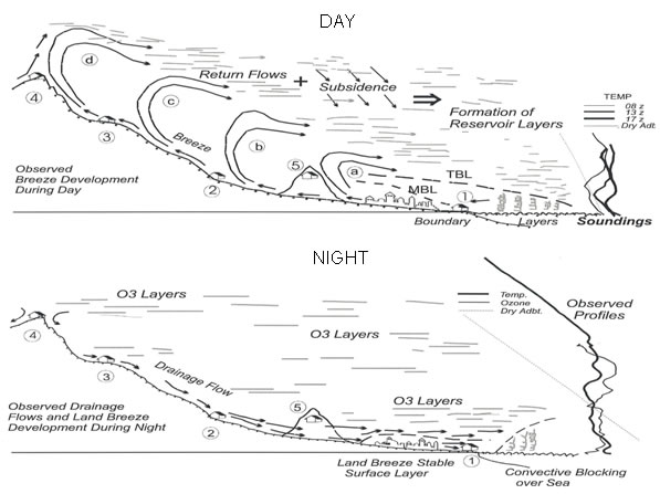
Figure 7.          Top:  Schematic of the atmospheric circulations in the coastal regions of the western Mediterranean on a summer day.  Letters a-d indicate successive stages in the entrance of the seabreeze and the formation of stratified layers aloft.  Bottom: The same for a summer night.  Soundings at right, from the MECAPIP project instrumented flights (0541-0546 UTC 20 Jul 1989) extending to 3500 m altitude, illustrate the stratification over the sea some 40 km offshore (see also Figure 8 for the temperature profile obtained during the previous leg of the same flight).  Common features in this and other soundings are: a quasi-isothermal, but strongly serrated, aspect in their lower » 2000 m, and a nearly adiabatic form in their upper parts.  The latter suggests the sustained subsidence of a well-mixed airmass and also supports the notion that the upper layers are formed at the last stage of penetration of the combined breeze, i.e., over the mountain tops, after the air in the combined breeze has become well mixed during its travel over the heated surface, and within the last orographic chimney.  At this point, the layer formation time is also the longest (4-6 hours).  Finally, the total amount of sinking experienced by these quasi-adiabatic layers (as illustrated in Figure 8) is comparable to the altitude of the ridges over which the injection took place (e.g., 1000 m to 1500 m).

Figure 8.          Top: Ozone (blue) and temperature (red) profiles measured over the Gulf of Valencia.  These illustrate the layers formed in the return flows of the coastal circulations.  Profiles A and B were obtained during the RECAPMA project (on July 16, 1991) over the points shown on the maps at right (blue triangles).  The faint black temperature profile was obtained over the same area during the MECAPIP project (0527 to 0541 UTC on July 20, 1989).  These illustrate how repetitive the coastal circulations can be over the Western Mediterranean Basin.  Bottom:  Out of 30 spiral flights, this overlay includes the profiles with the highest and the lowest potential temperatures observed in the return flows during the EC’s RECAPMA project in July 1991.   The values span the 312 K to 315 K range in the upper reaches of the flights, and the 24º C to 26º C range at the surface.  They suggest that the marine airmasses that enter the coastline at temperatures of  » 24° to 26° C gain from 13 K to 19 K by the time they become injected into the uppermost return flows aloft.  The red-dashed 303 K adiabatic profile (30ºC to 2000m) is a reference.

Figure  9.         Simulation of the temperature profiles for the places shown at right, at the times indicated.  The line with small red circles shows the modelling results at the UTC times indicated (full hour).  These are two cases where the modelling results clearly underestimate the temperature profiles measured by the instrumented aircraft.

Figure 10.  RAMS simulation of the wind field over the Mediterranean at 16:00 UTC on 19 July 1991.  At approximately the same time two spirals were flown up and down the red line over the red triangle marked south of Majorca (data in Figure 8, 315 K profile).  Top graph:  The winds at a height of 14.8 m emerge from the centre of the Western Basin and increase in speed while flowing anticyclonically (clockwise) towards convergence lines located over the main mountain ranges surrounding the basin (in orange).   Bottom:  The vertical component of the wind speed along the 39.5 North Parallel (dotted blue line in the upper graph) shows deep orographic-convective injections (black solid traces) over Eastern Spain and, following to the right, over Sardinia and the west-facing coasts of Italy, Greece and Turkey.  That is, to replace the surface air moving towards the coasts, continuity requires sinking of the air aloft, i.e., compensatory subsidence (dotted lines) over the seas. 

Figure  11.       Top left.  One of the experimental deployment areas used in nine EC projects in the Mediterranean. It marks the sounding sites for the other graphs (red arrows). Tethered balloons were used in a vertical profiling mode at the coast (PORT), at 20 km inland (SICHAR), and at 78 km inland (VALBONA).  The hourly evolution of the mixed layer at these sites, and the number of soundings used for the statistics are shown in each graph.  In each sounding, the height to the first observed temperature inversion was considered to be the boundary (mixed) layer depth.  The graphs show the average height of the BL (in blue) and the ± one standard deviation for each series.  Oscillations in the BL height had been previously observed in the 1978 Nanticoke Power Plant Experiment on the north shore of Lake Erie, Canada (Portelli et al. 1982).  In Valbona, the soundings were performed at selected time periods (early morning, afternoon, evening), instead of the half-hour cadence used on the other sites; hence, the observed gaps in the series.

Figure  12.       The summer shower/storm cycle on Western Mediterranean coasts.  Upper. Conditions in the past provided enough additional moisture to the marine airmass (seabreeze) to trigger precipitation almost every day at the » 1000 m altitude.  This kept a large amount of water recirculating within the coastal system, i.e., surface water and acquifers.  Note that the water evaporated at the coasts precipitates in the interior and, thus, that the real water cycle includes the acquifer that feeds the coastal marshes; i.e., they are all part of the same “water body”.  Lower.  Conditions with increased heating and less evapo-transpiration along (a drier) surface.  With an average heating of 16 K (see Figure 9), the marine airmass needs to accumulate a water vapour mixing ratio ³ 20 g/kg to bring the Convective Consensation Level below the 2000 m altitude, i.e., the approximate height of the coastal mountain ranges.  Under current conditions the average water vapour mixing ratio at the coast is »  14 g/km, and the contribution by surface evaporation along the path of the breeze is of the order of 5-6 g/km, which may not be enough to produce condensation and trigger a storm.   

Figure  13.       This figure from the TAR (IPCC 2001) synthesises the (idealized) development of Climate Models.  The second module includes Land surface interactions.  In the 4AR (IPCC 2007, 8.6.3.1 Water Vapour and Lapse Rate), it is stated that “In the planetary boundary layer, humidity is controlled by strong coupling with the surface, and a broad-scale quasi-unchanged RH response is uncontroversial”.  The uncontroversial part of this statement could be false for any region outside flat terrains in the mid latitudes.  The reason for this being that: when the edges of the continents wrap around a large interior sea like the Mediterranean, or a large semi-enclosed sea like the Sea of Japan, Continental Edge effects blend together to create their own large meso-meteorological circulation, particularly in summer.  These large meso-a scale circulations (to » 2000 km) can dominate the weather patterns in these regions for months, and include vertical recirculation cycles lasting several consecutive days.  Under these conditions, marine airmasses cross the coastline and become injected aloft over the mountains surrounding the sea.  This produces a systematic folding of surface boundary layers over the sea. The results are modified temperature profiles, i.e., the layers have gained potential temperature, as well as modified vertical water vapour distribution, since the layers now include the additional water evaporated over land.  The accumulation mode has been observed to reach 4500(+) m) over the enclosed Mediterranean Sea, and a similar process could also occur over other semi-enclosed large basins (Sea of Japan, South China Sea) in the subtropical latitudes.

                    DAY                                                                               DAY + NIGHT

Figure 14    Averages of the NASA MODIS-Terra measurements for July 2000 and 2005.   The Day product derived from the morning pass at 10:30 UTC emphasises the areas where the satellite looks down the deep orographic-convection developing at the fronts of the combined up-slope and seabreezes, i.e., around the edges of the basin (Figures 6, 7, and 10). It also outlines the deep inland penetration of the seabreezes over the desert areas of Tunisia, Libya and Egypt.  The Day+Night product emphasises the areas over which water vapour accumulation occurs at the end of the diurnal cycle.  That is, the water vapour that did not precipitate over the coastal mountains in the afternoon returns with the flows aloft and fills the Western Mediterranean Basin (to 4500 + m) and the Adriatic and Black seas with water vapour (layers).  This produces an “accumulation mode” in summer and, without requiring the high evaporation rates of more tropical latitudes, the mechanisms described in the text are able, in just a few days, to generate a very large, deep and polluted air mass that increases both in moisture content and in potential instability with each passing day.   The vertical circulation accumulation cycle can last for several days (i.e., 4 on the average and periods of up to 7 or more) and recur several times per month (up to 12 to 24 days in July-August).  As a result, the monthly averages shown here are comparable to the column values of water vapour accumulated after 4 days of vertical recirculations.

.

Comments Off on Guest Post – Climate Change Predictions, Including Extreme Hydrometeorological Events By Dr. Millán Millán

Filed under Guest Weblogs

“The Greenhouse Effect – Part II” by Ben Herman and Roger Pielke Sr.

Update #2 John Nielsen-Gamon has alerted us to more information on the Moon’s radiative temperature. John e-mailed

 I read your blog post on Greenhouse Part 2.  I also recently came across the Science of Doom web site; it seems to be of very high quality.  You might want to link to http://scienceofdoom.com/2010/06/03/lunar-madness-and-physics-basics/ [on] your post to direct the reader to further details on the radiative temperature of the Moon.

Update – corrected text (underlined) h/t to Gerald E. Quindry

We have received a further question on our post

“The Greenhouse Effect” by Ben Herman and Roger Pielke Sr.

The question is summarized by the following text

Anyway my question refers to the common example of taking away the atmosphere and observing a cold surface. But as I understand it, the mean daytime surface temperature on the moon is over 100 C, with no  greenhouse effect. The mean nighttime temp drops to -150 C. http://www.solarviews.com/eng/moon.htm

This is important to note, because encouraging a popular picture in which the presence of the atmosphere only warms the surface takes all the convection and fluid dynamics out of the discussion, and that’s where all the important complexities are.

Isn’t it more the case that the atmosphere both warms and cools the surface, depending on circumstances? The IR absorption of H2O and other GHG’s warms the surface relative to what it would otherwise be, but as the lunar case shows, convection and turbulent mixing cools the surface relative to what would happen without an atmosphere. Take away the atmosphere and you take away both warming and cooling mechanisms.

We have reproduced the substance of our follow up answer below.

Predicting the surface temperature indeed involves the interaction of the atmospheric and ocean turbulent sensible and latent fluxes, long- and short- wave radiative fluxes and interfacial fluxes between the surface and the atmosphere. I have been urging for years to move away from the surface temperature to characterize global warming and cooling (and replace with ocean heat content changes in Joules) because the surface temperature is such a limited sample of the heat content changes of the climate system as well as involving these complicated feedbacks.

 On the Moon, there is, of course, no atmosphere, so its surface temperature results from the difference between the surface long wave radiative emissions, the amount of solar radiation absorbed and reflected, and the conduction of heat into and out of the surface. The effect of the atmosphere on Earth is to mute the diurnal (and seasonal) temperature range as a result of the turbulent fluxes, and other effects (such as clouds and precipitation). These atmospheric effects, for example, result in lower daytime and higher nighttime temperatures from what they otherwise would be. I presume this is the cooling and warming effects that you refer to. However, even with these effects, the surface is clearly warmer than it would be without the CO2 and water vapor IR absorption bands.

But the reasons are that the atmosphere scatters back to space some sunlight, and takes up some of the surface heating through conduction, and mixes it it by convection and turbulence. Also, the relatively rapid rotation of the earth on its axis  does not permit the daytime side to reach equilibrium before it starts nighttime cooling. As a result, daytime temperatures on earth are cooler than they would be with no atmosphere, and warmer at night than with no atmosphere.

Of course, the Moon, with no atmosphere, still  has to have basically the same effective radiating temperature as does the Earth. This should be

[sigma *Tmd**4 + sigma* Tmn**4]/2 = sigma*Te**4  where Tmd is the daytime temperature of of the Moon, Tmn is the night time temperature of the Moon, and Te is the effective radiating temperature of the Earth.

The fact that the daytime time temperature is warmer than the Earth’s temp is simply a result of the fact that the Moon is not in an equilibrium state – it warms up during the daytime and cools down at night, just as does the Earth. However the warming during day and cooling at night must balance each other or the Moon ( and the Earth) would be steadily heating up or cooling down over time.  The daytime warming occurs because the outgoing IR cannot balance the absorbed solar during the day. The nighttime cooling occurs because the outgoing IR is greater than the non-existing solar at night. The existence of a partially absorbing atmosphere does, as you stated, keep days cooler and nights warmer.

Also, the length of a day on the Moon is 29.5 earth days, almost a full Earth month. Therefore the daylight side of the Moon heats due to solar radiation, for half a month. Then when it’s night, it cools for another half month. Thus the daytime and nighttime temperatures are much more extreme. There is no greenhouse effect on the Moon, of course, and if the Moon’s day was the same 24 hours as an Earth day, its day and night temperatures would not vary  as much but its  radiative equilibrium temperature would be the same.

Comments Off on “The Greenhouse Effect – Part II” by Ben Herman and Roger Pielke Sr.

Filed under Climate Change Forcings & Feedbacks, Guest Weblogs

Guest Post “Calculating Moist Enthalpy From Usual Meteorological Measurements By Francis Massen

Francis Massen, in response to the posts,

Comment On The Northeast Heat Wave

Further Information On The Role Of Water Vapor In Measuring Heat By Francis Massen

has graciously prepared a write up of how to compute the moist enthalpy of surface air. Francis websites include http://meteo.lcd.lu/; http://computarium.lcd.lu/; and http://bmb.lcd.lu/

Calculating Moist Enthalpy From Usual Meteorological Measurements By Francis Massen

Abstract: This short article shows how to compute the moist enthalpy from usual meteorological measurements of dry temperature, air pressure and relative humidity. The result is used to add a plot of moist air enthalpy to the other near-live graphs shown by meteoLCD, the meteorological station of the LCD, Diekirch, Luxembourg

1. Sensible heat of dry air

The sensible heat of dry air is defined as Ha = Cp*T [ref. 3] with Cp usually taken as 1.005 when Ha is given in [kJ/kg] and temperature T in [°C].

Here we will use for Cp the following expression, valid for temperatures higher than 0 °C and lower than 60 °C, as given by PADFIELD [ref.2]

Ha = 1.007*T – 0.026          0 °C < T < 60 °C                                                         [eq.1]

2. Heat content of water vapor at temperature T

The heat content of water vapor is the sum of the latent heat of vaporization and the sensible heat of water vapor:

Hv =  q*( L + 1.84*T) [ref. TET]                                                                               [eq.2]

Where L = heat of vaporization = 2501 kJ/kg at 0°C

and 1.84*T = sensible heat of water vapor in kJ/kg

The sensible heat term of eq.3 (1.84*T) is very often considered negligible and omitted. 

Note:L is a function of temperature, becoming slightly smaller with increasing T; for values between 0°C and 50°C one can use the linear interpolation L(T) = 2502 – 2.378*T computed by the author from a table with enthalpy values given by YHCHEN [ref.4]: The linear fit is excellent with R2 = 0.9998.

Combining eq.2 with L(T) gives:

Hv = q*(2502 – 0.538*T)    with Hv in kJ/kg and T in °C                [eq.3]

3. Total enthalpy of moist air

Total enthalpy of moist air is the sum of Ha and Hv:

H = Ha + Hv = (1.007*T -0.026) + q*(2502 – 0.538*T)                       [eq.4] 

with H in kJ/kg, T in °C and specific humidity q in kg/kg

The problem with this formula is that the specific humidity q is usually not measured by a standard meteorological equipment which commonly measures relative humidity.

4. Finding q from measured dry bulb temperature, relative humidity and atmospheric pressure

PIELKE [ref.3] and the AOMIP website [ref.1] give the following formula for the specific humidity q:

                                          [eq.5]

where ea = vapor pressure in [Pa] and pa = atmospheric pressure in [Pa].
Attention: pa is the true air pressure, not the barometric pressure reduced to sea level!

Dividing numerator and denominator by ea gives:

                                                               [eq.6]

Relative humidity is the fraction of water vapor pressure to saturated water vapor pressure, usually multiplied by 100 to give a percent value:

RH = 100* ea/esat  →  ea = RH/100*esat

There are many different formulas relating esat to temperature. We will use the expression given in AOMIP [ref.1] and valid up to 40°C:

       [eq.7]

with saturated water vapor pressure esat in [Pa] and temperature T in °C.

Equations 4, 6 and 7 contain only T, RH and pa, which are parameters measured by practically every standard weather station. Together they can be used to calculate the enthalpy of moist air by a single (albeit unwieldy) formula:

          [eq.8]

This expression is valid for temperatures 0°C < T < 40°C. Units: H[kJ/kg], T[°C], pa[Pa] 

5. A practical example

The author has used eq.8  in GNUPLOT to display near-live plots of the moist enthalpy at meteoLCD, Diekirch, Luxembourg (see http://meteo.lcd.lu/today_01.html). The following figure shows the situation for the week from 10 to 16th July 2010. Sensible heat is shown by the blue bottom curve; the difference between the upper red curve ( = moist enthalpy) and the blue curve corresponds to the latent heat.

Technisolve Software has a website with an online moist air calculator, which is very handy for a quick validation check of individual values: http://www.coolit.co.za/airstate/airmoistobject.htm

References

[1] AOMIP: Atmospheric Forcing Data – Humidity

http://efdl.cims.nyu.edu/project_aomip/forcing_data/atmosphere/humidity.html

[2] PADFIELD, Tim: Conservation Physics

 http://www.conservationphysics.org/atmcalc/atmoclc1.php

[3] PIELKE, Roger, Sr., WOLTER, Klaus: The July 2005 Denver Heat Wave: How unusual was it ?. National Weather Digest, vol.31, no. 1, July 2007

http://pielkeclimatesciencesci.files.wordpress.com/2009/10/r-313.pdf

[4] TET (The Engineering Toolbox)

http://www.engineeringtoolbox.com/enthalpy-moist-air-d_683.html

[5] YHCHEN: Calculation of Enthalpy Changes

www.ntut.edu.tw/~yhchen1/Chap.%2023.pdf

Comments Off on Guest Post “Calculating Moist Enthalpy From Usual Meteorological Measurements By Francis Massen

Filed under Climate Change Metrics, Guest Weblogs

Climate Change: The West vs The Rest by Will Alexander

We are fortunate to have a guest post by Will Alexander (see his earlier one here). WJR (Will) Alexander is Professor Emeritus of the Department of Civil Engineering of the University of Pretoria, South Africa, and Honorary Fellow of the South African Institution of Civil Engineering. He spent the past 35 years of his career actively involved in the development of water resource and flood analysis methods as well as in natural disaster mitigation studies. His interest in climate change arose from claims that it would have an adverse effect in these fields. In his subsequent studies of very large hydrometeorological data sets he was unable to detect any adverse human-related changes. He has written more than 200 papers, presentations and books on these subjects. [alexwjr@iafrica.com]

GUEST POST By Will Alexander

Disarray

Climate change is presently in a position of total disarray. The credibility of many scientists and their institutions is at risk. It is not difficult to identify the origin of the problem.

The G20 and G8 nations are due to meet in Canada during June. The United Nations Secretary General visited Canada during May. His mission was to convince the Canadian Prime Minister to elevate climate change above the global economic crisis to the top of their agenda. The request was refused. This was an amazing request.

The global financial crisis is adversely affecting the livelihoods of many millions of people across the world. It has its origins in the financial mismanagement of the Western nations. What the Secretary General, his advisers and the Western nations failed to realise is that this whole climate change charade has its origins in a decision made by the G8 nations at a meeting at Glen Eagles, Scotland in June 2005. This is what happened.

The international academies of science produced a document: Joint science academies statement: global response to climate change. It was addressed to the G8 nations’ summit meeting. The signatories accepted the IPCC’s assessment reports of 2001, and then made further recommendations.

I draw your attention to its comments that adaptation to climate change required worldwide collaborative inputs from a wide range of experts, including physical and natural scientists, engineers, social scientists, medical scientists, those in the humanities, business leaders and economists. [ This recommendation was ignored.]

Also note the following important paragraph.

Work with developing nations to build a scientific and technological capacity suited to the circumstances, enabling them to develop innovative solutions to mitigate and adapt to the adverse effects of climate change, while explicitly recognizing their legitimate development rights. (My emphasis). [This recommendation was also flagrantly ignored. In the years that followed all nations of the world, east and west, rich and poor, were expected to follow this suicidal path.]

The Stern Review

The academies’ recommendations to the G8 nations resulted in the appointment of Nicholas Stern, a British senior civil servant and economist to review the whole climate change issue and make recommendations. After his appointment he called for submissions.

I responded to his request. On 24 November 2005 I submitted my 92-page technical report An assessment of the likely consequences of global warming on the climate of South Africa as well as my United Nations commissioned report Risk and society — an African perspective. They were ignored.

On 20 February 2006 I responded to another call for comments. It was ignored as were my subsequent e-mails of 5 March and 13 April. I protested and offered to come to the United Kingdom and address a meeting of experts of his choice. It was also ignored. The original correspondence and my reports should be available in the archives of the Stern Review. Note the following passage in my e-mail of 13 April in particular.

Current climate change theory and the conclusions drawn from it are seriously in error. Governments that accept the IPCC’s position should be aware of this. They should also carefully consider the sociological, economic and political consequences should they undertake costly and economically restrictive measures that are subsequently found to be based on erroneous science. Climate change scientists should also be aware of the potential harm to tens of millions of the poor and disadvantaged people of the world should their recommendations be implemented and later found to be in error. They should also consider the risks to their reputations and to those of science and scientists in general. I’m very confident of my conclusions.

Alas, these predictions have come to pass.

The brief notes below illustrate one of the many examples in my report to the Stern Review that completely demolishes the alarmist predictions by climate change scientists as described in the IPCC’s assessment reports.

The fourth assessment report was published in segments during 2007. The following sentence was published in the report. The same view was also expressed in earlier assessment reports.

The human activity on climate in this era greatly exceeds that due to known changes in natural processes, such as solar changes and volcanic eruptions.

This single statement lies at the very core of the whole climate change charade.

Solar linkage

In the 1850s British astronomers reported the linkage between sunspot numbers and famines in India. In 1889 D.E. Hutchins published his book Cycles of drought and good seasons in South Africa. He based his analyses on data from the Royal Observatory in Cape Town that was established in 1842. In the 1960s through to the 1980s engineering hydrologists became increasingly concerned about the unexplained variability present in many hydrological records. In the 1960s there were already references to the receipt and poleward redistribution of solar energy as the probable driver of these variations. I was directly involved in international discussions on these serious hydrological anomalies from 1970 onwards.

Over the years I produced approximately 3 GB of calculations, technical reports and refereed publications on this subject. One of these was my extended summary report that I submitted to the Stern Review in November 2005. My report was titled An assessment of the likely consequences of global warming on the climate of South Africa. It had 92 pages, 15 figures, 13 tables, and 50 references. I was aware of the requirements expressed by the international academies of science at that time. My report was directly relevant to the recommendations by the academies.

The essence of my report was that after three years of study of a comprehensive hydrometeorological database, I could find no evidence of unexplained variations in the data. It became increasingly obvious that the anomalies were the consequence of variations in the receipt and poleward redistribution of solar energy.

Subsequently my reports and papers were targeted at South African readers. I had lost all faith in material published by Western authors in the light of my experience with the Stern Review. It was impossible to determine the nature of material that was deliberately omitted from their analyses, as well as the deliberately manipulated data such as that produced by the Climate Research Unit of the University of East Anglia in the UK.

The following are very small samples of the figures and tables in my report. Table 1 is the comprehensive and extensive database used in the analyses. It is available in computer-readable format.

Table 1.  Database used in the analyses
Set Process Stations Years
1 Water surface evaporation 20 1180
2 Concurrent rainfall 20 1180
3 District rainfall 93 7141
4 Dam inflow 14 825
5 River flow 14 1052
6 Flood peak maxima 17 1235
7 Groundwater 4 312
8 Southern oscillation index 1 114
  TOTAL 183 11 804

Figure 9 is very important. It demonstrates the unequivocal synchronous relationship between annual sunspot numbers and the annual flows in the Vaal River that is South Africa’s major river. Note the alternating above (rising) and below (falling) flow sequences. Note also their synchronous relationship with sunspot numbers; as well as the statistically significant (95%), 21-year periodicity in the flow data that is synchronous with the double sunspot cycle.

Notice also the absence of 11-year periodicity in the correlogram of the Vaal River. It is no wonder that climate change scientists have been unable to detect synchronous relationships with the 11-year sunspot cycle. It does not exist! This is because the properties of the alternating solar cycles are fundamentally different to the extent that the climatic responses are also very different.

Figure 9. Comparisons of the characteristics of annual sunspot numbers with corresponding characteristics of the annual flows in the Vaal River.

Another frequent error associated with the sunspot cycle is the assumption that the maximum effect is associated with the sunspot maxima. This is altogether wrong. The maxima occur immediately after the solar minima. Table 10 illustrates this.

Table 10. Comparison of sudden changes in the annual flows in the Vaal River with corresponding sudden changes in sunspot numbers
Three-year totals of flows in Vaal River (% of record mean) Three-year totals associated with the corresponding sunspot minimum
Minimum year Three previous years Three subsequent years Sunspot minimum Three lowest years Three subsequent years
1932/33 100 388 1933 25 250
1941/42 297 625 1944 56 277
1953/54 205 538 1954 50 370
1965/66 234 241 1964 53 247
1972/73 177 654 1975 73 275
1986/87 112 438 1986 60 400
1994/95 135 464+ 1996 48 277
Average 180 478 Average 52 300


Table 12 demonstrates the well-known Joseph Effect of alternating above and below average multi-year sequences published separately by two other South African authors. It is very interesting. Compare the durations of the wet and dry sequences with Josephs biblical prophecy of seven years of plenty followed by seven years of famine. The coincidence is not fortuitous.

Table 12. Wet and dry sequences
Years Wet/dry Length of sequence Sunspot cycles
    Wet Dry  
Bredenkamp:   Mzimgazi + St Lucia + Uitenhage + Wondergat
1919-24 Wet 5   1913-22
1925-29 Dry   4 1923-32
1930-39 Wet 9   1933-43
1941-53 Dry   12 1944-53
1955-62 Wet 7   1954-63
1965-71 Dry   6 1964-75
1972-78 Wet 6   1976-85
1980-83 Dry   3 -do-
1984-90 Wet 6    
Tyson: South African rainfall
1905-15 Dry   10 1901-12
1916-24 Wet 8   1913-22
1925-32 Dry   7 1923-32
1933-43 Wet 10   1933-43
1944-52 Dry   8 1944-53
1953-61 Wet 8   1954-63
1962-70 Dry   8 1964-75
1971-80 Wet 9   1976-85

This table completely destroys the repeatedly stated claim in the IPCC literature that there is no meaningful linkage between variations in solar activity and synchronous linkages with variations in the climatic processes.

Conclusions

The following conclusions were summarised on the first page of my report.

Continued global warming will NOT

  • Pose a threat to water supplies
    • Adversely affect agricultural production
  • Increase the risk of floods and droughts
  • Increase the spread of malaria
  • Increase the eutrophication of water in dams
  • Increase soil erosion
  • Result in the loss of natural plant and animal species
  • Result in desertification

There is no believable evidence to support these claims.

It would be most unwise

For South African authorities to force the implementation of costly measures, based on unverifiable global climate models, and abstract theory, for which there is no believable evidence.

References

My technical report contained 50 references. The following are seven references to my prior publications in scientific journals. They were therefore available to the Stern Review.

Alexander W J R 1985. Hydrology of low latitude southern hemisphere landmasses. In Hydrobiologia, ed Davies & Walmsley, Junk Publishers, Holland.

Alexander W J R 1995. Floods, droughts and climate change. South African Journal of Science 91, 403-408.

Alexander W J R 1999. Risk and society – an African perspective. United Nations commissioned study. Geneva, Switzerland.

Alexander W J R 2002a. Climate change – the missing links. Science in Africa. September 2002.

Alexander W J R 2002b. Statistical analysis of extreme floods. Journal of the South African Institution of Civil Engineering, 44 (1) 2002 20-25.

Alexander W J R (2005a). Development of a multi-year climate prediction model. Water SA Vol 31 No 2 April 2005.

Alexander W J R (2005b) Linkages between Solar Activity and Climatic Responses. Energy & Environment, Volume 16, No 2, 2005.

Finally

Why was my report deliberately ignored by the Stern Review despite my protests and offers to come to the UK to present it to a critical audience of his choice? There can only be one answer. It completely undermines the claim is of exclusive human causality of climate change. Now the whole climate change issue is in total disarray as a consequence of this demonstrably false assumption.

Many scientists in other fields have reported similar experiences. It is now very clear that the manipulation of science in the IPCC publications was a general practice. There are increasing suspicions that these manipulations were intended to force developing nations to undertake costly measures that would reduce their rising economic competitiveness with the West. The failure of the World Trade Organisation to produce a binding international agreement is also a consequence of Western nations protecting their own interests.

The situation is very fluid. China has already overtaken the Western nations as Africa’s major trading partner. This is one battle that the West cannot win.

I’m prepared to e-mail a copy of my technical report and the data used in the analyses in computer readable format, with my compliments to anybody who has an interest.

W.J.R. Alexander Pr Eng

Professor Emeritus, Department of Civil Engineering, University of Pretoria, South Africa.

Fellow, South African Institution of Civil Engineering

Member, United Nations Scientific and Technical Committee on Natural Disasters, 1994 – 2000

Email alexwjr@iafrica.com

Comments Off on Climate Change: The West vs The Rest by Will Alexander

Filed under Guest Weblogs

Further Comment By Kevin Trenberth

On Sunday April 25 2010, Kevin sent me the e-mail below which continues the constructive discussion we are having on Climate Science.  It is reproduced below with his permission.

Roger

I am just back from travel: actually I was at a mtg in Atlanta with your son!

I saw Roy Spencer’s comment for the first time and it is not correct.  The CERES data are indeed processed to give the reflected solar radiation and outgoing longwave radiation, which combine to give the net radiation.  The biggest single change, which occurred abruptly, is a drop in OLR at the beginning of January 2008 and lasting throughout most of 2009 with only a brief return to “normal”.  Values are between 0.5 and 1 W m-2 below the normal which is the mean for the record from 2000 through about 2005 (I think) and thus not normal in the sense of being radiatively balanced (the zero is not a true zero).  On the other hand, the reflected solar is higher from 2000 through 2003, and runs up to about 0.5 W m-2 below the mean thereafter.

The abrupt nature of the drop in OLR made it look very suspicious to me and we looked at the daily values.  The drop seems to occur very near the start of 2008. We have raised this with the CERES team who find that it is replicated in a separate measurement from AIRS data.  It occurs during La Nina and is thus consistent with changes in high cloud (more cloud), which has some plausibility.  We explored the cloud records from three sources but all disagree and the quality of cloud information is not yet good enough for this sort of thing.  Fortunately cloud data (ISCCP) are being reprocessed.  However, definition of cloud and changes in sensitivity of the instruments are difficult challenges.  The more sensitive the instrument, the more cloud is found, even though it is very thin.

We hope that our paper is a stimulus to help improve the records of all aspects of this problem, the radiation , the ocean heat, and the way they are processed.

Kevin

I am inviting Roy to respond to Kevin’s comment.

Comments Off on Further Comment By Kevin Trenberth

Filed under Climate Change Forcings & Feedbacks, Guest Weblogs

Living on the Edge – Changing Wetlands in the Sahel – A Book Review by Henk Tennekes

Dear friends in the blogosphere, I received a precious gift from a Dutch friend a little while ago. Living on the Edge: Wetlands and Birds in a Changing Sahel is a massive book, comprising 564 pages in full color and countless stunning photographs (see footnote for publication details). The tragic story of the Senegal River Delta described in this book reminded me of Roger Pielke’s studies of climate change in Florida, caused by the drainage of swamps and the southward march of citrus plantations over the last century. In 1985, I saw with my own eyes how the River Jordan is drained to a trickle flow to irrigate the fertile soil at the foot of the Carmel Ridge. I know of the enormous amount of water drained from the Colorado River to irrigate California’s Central  Imperial Valley, and, like many others, I worry what will happen to the western prairie states after the Ogallala Aquifer, from which 26 billion cubic meters of water is extracted annually, has been depleted.

There is much more to climate change than the rallying cries about Global Warming suggest. Nowhere is this made clearer than in the Sahel, a narrow strip of African countryside between the Sahara Desert in the North and the rain forest along the Gulf of Guinea in the south. The annual rainfall in the Sahara is only 20 millimeters, but 400 kilometers to the south the annual precipitation reaches 2000 millimeters or more. In the Sahel, plants, animals and people live on the edge of what is ecologically sustainable. Living on the edge of the cliff, as it were. The title of the book projects an apocalyptic image.

This problem became acute around 1965, when the entire Sahel threatened to succumb to desertification. No one less than Jule Charney, the great meteorologist we all admired, studied this issue in great detail. In conversations with George Platzman, he said : “at that time we were getting news of the terrible drought in the Sahel, and it occurred to me that the overgrazing, which I ascertained occurred over an enormous area – I mean the cow, since there’s very little forage in the first place, could crop whatever brush or grass exists over an enormous area, that it was not unreasonable to take an area the order of 400 kilometers in the north-south direction, and going across the whole Sahara …. I proposed to Jastrow and Halem at the Institute for Space Studies that they should take their model and simply raise the albedo over this particular strip and see what happened. And indeed, that resulted in a about a forty or fifty percent reduction in rainfall. And there I became interested in the general climatological question of how alteration of surface properties could influence regional climate. It is not only albedo, but also soil moisture, because evaporation is a very important thing” …. (pp. 78-79 in The Atmosphere – A Challenge, AMS 1990).

Fortunately, the threatening desertification proved to be reversible. Rainfall increased again after 1973, and the Sahel also survived a second dry period, between 1981 and 1987. The nightmare of the mid-eighties is still imprinted on my friend’s retina. The media focused on the hardship for the local people, and their struggle for life, but the authors of Living on the Edge describe the devastating impact of drought on migratory birds. Breeding from Greenland to Siberia and wintering in the Sahel, these include more than a hundred species and 4,500 millions of individuals. Within the last 40 years we have lost at least a third of that population. Apocalyptic numbers, but people, members of that superior species, don’t seem to care.

Tales of alternating dry and fertile periods made me think of Egypt’s viceroy Joseph, who implemented a cereal storage system to ride out seven lean years in similar climatological conditions 3600 years ago. The bibliography of Living on the Edge contains several recent papers by Latif, Palmer, Hulme, and others that deal with possible causes for this periodicity. It appears that the surface temperatures of the tropical oceans surrounding Africa strongly affect Sahel rainfall. The meridional temperature gradients in the Atlantic and Indian oceans exert some influence, too. In any case, Hulme (2001) concluded that rainfall in the western Sahel may decrease 20% or more in the foreseeable future. Prospects are bleak.

The Sahel suffers from a confluence of threats to its people and its ecosystem. Explosive population growth, 3% or more annually, will overwhelm the scarce resources of the region before too long. Imported cereals are needed as it stands; the rapid expansion of irrigated rice fields cannot keep up. Floodplains, havens for millions of migratory birds, are disappearing fast. The progress of urbanization makes matters worse: city dwellers aspire to mimic the consumption patterns of people in the industrial world. Malaria is rampant, thanks to the ban on DDT. The delta of the Senegal River has been tamed by dams and levees twenty times as fast as the delta of the River Rhine, where I live. The Niger River suffers a similar fate. Four countries border on Lake Chad; no politician there seems to care about its future.

Living on the Edge describes the fate of twenty-seven species of birds in detail. For this review I will focus on White Storks (Ciconia ciconia). When they arrive in the Sahel in fall, the rainy season has just ended and there is an abundant food supply. Storks forage voraciously then, adding a kilogram of fat to their 3.5 kg bodies. One would think they are fattening up in preparation for their return trip, but they are not. They are preparing themselves for the dry months of early spring, in which the food shortage can become severe if the ITCZ shifts position too early. In a bad year, they are in far less than optimal condition when they have to cross the Sahara on their way back to their European breeding grounds. That can lead to massive mortality. Typically, 25% of juveniles die on their way back. Another 25% is killed in collision with high-voltage power lines, mainly in Spain. The mortality from that cause alone is 4 birds per kilometer per year.

I will never forget one horrible detail that I came across in the book. Fat birds are excellent sources of protein and lipids, so locals hunt them with a vengeance. Storks are soaring birds, with relatively weak flight muscles. Fattened up, they are an easy prey. So what do the locals do? They break the arm bones of these birds, so they can’t fly anymore. Broken wings – a nightmare. Subsequently, the captured storks are kept as pets, until they are wanted in the frying pan. Such customs, however excusable in a situation with scarce food supplies, make one ashamed of belonging to the human race. The treatment of animals in the meat industry of Eurasia and both Americas is far worse.

Living on the Edge details an ecological nightmare. It never fails to grip my throat whenever I am browsing through. Comparing this book with the thousands of pages produced by IPCC every five years, full of abstract intellectual exercises and bureaucratic theorizing, I realize better than ever before what the principal shortcoming of the “traveling climate circus” is. The crowd that follows IPCC lacks empathy. Global Warming is a cocktail-party hobby of well-educated city dwellers in Europe and elsewhere, people who cannot imagine the life of a farmhand in India or Senegal, people who do not contemplate the suffering of a stork with broken wings.

On Mary Black’s album “Speaking with the Angel” are these lyrics:

But these broken wings won’t fly
These broken wings won’t fly
These broken wings won’t fly at all

And oh how we laugh but maybe we should crawl
And ask to be excused
We shout loudly, have answers to it all
Oh but we have been refused

Yes, IPCC adherents shout loudly, and have answers to it all. Perhaps they should ask to be excused for not realizing that all of us are Living on the Edge, not just the people and the birds in the Sahel.

FootnoteLiving at the Edge – Wetlands and Birds in a Changing Sahel, by Leo Zwarts, Rob Bijlsma, Jan van der Kamp, and Eddy Wymenga (2009, ISBN 978 90 5011 280 2) is published by KNNV Publishing, Zeist, Netherlands (www.knnvpublishing.nl). The book is not cheap: approximately $85. Keep your credit card ready.

Comments Off on Living on the Edge – Changing Wetlands in the Sahel – A Book Review by Henk Tennekes

Filed under Books, Guest Weblogs

Guest Post By Thomas Chase On An Update On “Was The 2003 European Heat Wave Unusual In A Global Context”

Guest Post By Thomas N. Chase

Update on

Chase, T.N., K. Wolter, R.A. Pielke Sr., and Ichtiaque Rasool, 2006: Was the 2003 European summer heat wave unusual in a global context? Geophys. Res. Lett., 33, L23709, doi:10.1029/2006GL027470.

In Chase et al. (2006) we documented the June, July, and August averaged thickness temperature anomalies in terms of standard deviations exceeded and concluded that, while the European heatwave was unusual, natural variability in terms of ENSO and volcanic eruptions exceeded the extremes of the European heatwave. In subsequent commentary on this paper, Connelly (2006) found that the European heat wave was indeed quite unusual if surface temperature data was used prompting Chase et al. (2008) to conclude, along with others, that the unusual heat wave was confined near the surface was the result of surface processes and not a general warming of the troposphere as would be expected in a global warming scenario. We also concluded that with the updated time series that an upward trend in extreme variability was starting to appear. 

Here we update the original time series through 2009 as shown in Figures 1a,b,c which show the percentage of the Northern Hemisphere extratropics affected by 2.0, 3.0, and 3.5 SD anomalies, respectively. There is now a clear and significant upward trend in the most extreme variability (Table 1) with the summer of 2008 being the most extreme yet. This is due to very large warm anomalies in northeastern Canada, around Greenland, and also in Siberia (Figure 2). Interestingly, these extremes in SD exceeded are largest in the near-surface layers of the atmosphere than in the mid-troposphere despite the temperature variability at high latitudes being much larger near the surface than in the mid troposphere (e.g., Peixoto and Oort, 1992; Figure 7.8) again suggesting that surface processes are more responsible than generalized climate warming.  

Massive Arctic sea ice melt was likely one component of the unusual near-surface climate in Canada, the Labrador/Baffin Seas, and Greenland.


2.0 SD                              

 3.0 SD                                      

 3.5 SD          

Figure 1. Histograms of percentage of the Northern Hemisphere from 22-80°N covered by thickness temperature anomalies exceeding 2.0, 3.0, and 3.5 standard deviations, respectively. Cold anomalies are in dashed lines, warm anomalies in solid lines. Note the different vertical scales.

Figure 2. Thickness temperature anomalies 1000-500 mb for JJA 2008 (color shaded) and standard deviations exceeded (2.0, 3.0, 3.5, 4.0 SD) contoured.

Figure 3. Major Northern Hemisphere warm temperature anomalies by pressure level: 68°W, 57°N is the eastern Canada Greenland anomaly, 140°E, 63°N is the Siberian anomaly, 73°E, 35°N is the central Asia anomaly.

SD Exceeded Slope (%/year) P-Value
2.0 warm 0.152 0.01
3.0 warm 0.015 0.02
3.5 warm 0.003 (3 data points) 0.06
2.0 cold -0.998 0.11

 Table 1: Slopes and P-values for linear regressions for time series in Figure 1 and for 2.0 SD cold anomalies (not pictured in Figure 1). Higher-order cold anomalies are data sparse and are not given. 3.5 warm anomalies are also data sparse and not reliable (3 values) and are given only for completeness.

References

Chase, T. N., K. Wolter, R. A. Pielke, Sr., and I. Rasool, 2008. Reply to comment by W. M. Connolley on; Was the 2003 European summer heat wave unusual in a global context? Geophys. Res. Lett., 35, L02704, doi:10.1029/2007GL031574.

Chase, T. N., K. Wolter, R. A. Pielke, Sr., and I. Rasool, 2006. Was the 2003 European summer heat wave unusual in a global context? Geophys. Res. Lett., 33, L23709, doi:10.1029/2006GL027470.

Connelly, W.M., 2008. Comment on: “Was the 2003 European summer heat wave unusual in a global context?” Geophys. Res. Lett., 35, L02703,  doi: 10.1029/2007GL031171.

Peixoto, J. P., and A.H Oort, 1992. Physics of Climate. American Institute of Physics. New York.

Comments Off on Guest Post By Thomas Chase On An Update On “Was The 2003 European Heat Wave Unusual In A Global Context”

Filed under Climate Change Metrics, Guest Weblogs

Guest Post By Andrew Dessler On The Water Vapor Feedback

Professor Andrew Dessler of the Department of Atmospheric Sciences of Texas A&M University requested the opportunity to respond to my post

Q & A Are Water Vapor Feedbacks From Added CO2 Well Understood?

I welcome his openess to discuss this issue, and am glad to post his guest weblog. We need more such collegial debate on these topics within the climate community. I will respond in an upcoming post.

Guest Weblog By Andrew Dressler

In a recent post, Prof. Pielke emphasized the uncertainties in our knowledge of the water vapor feedback. In doing so, he failed to recognize the many things that are confidently known about the water vapor feedback.

There are really two questions here: 1) do observations indicate that the water vapor feedback strong and positive, and 2) do models adequately reproduce the observed feedback?

For the first question, the evidence of a strong and positive water vapor feedback is overwhelming. Observations of the response of the atmosphere to events like the eruption of Mount Pinatubo and El Niño cycles show quite clearly that changes in water vapor lead to enhanced trapping of infrared radiation when the climate warms [Soden et al., 2002; Soden et al., 2005; Forster and Collins, 2004; Dessler et al., 2008].  For a more complete summary of why we’re so confident, see Dessler et al. [2009]

It is particularly worth noting that the papers that Prof. Pielke referenced by Dr. Sun and colleagues (which he says casts doubt on models’ ability to simulate the feedback) clearly confirm with observations that the water vapor feedback is strong and positive. 

Given the strong water vapor feedback seen in observations (~2 W/m2/K), combined with estimates of the smaller ice-albedo and lapse rate feedbacks, we can estimate warming over the next century will be several degrees Celsius.  You do not need a climate model to reach this conclusion — you can do a simple estimate using the observed estimates of the feedbacks along with an expectation that increases in carbon dioxide will result in an increase in radiative forcing of a few watts per square meter.

The only way that a large warming will not occur in the face of these radiative forcing is if some presently unknown negative feedback that cancels the water vapor feedback.  My opinion is that the cloud feedback is the only place where such a large negative feedback can lurk.  If it is not there, and the planet does not reduce emissions, then get ready for a much warmer climate.

This brings us to the second question, whether models adequately simulate the feedback.

To investigate this, I have recently compared the global-average radiative response to changes in water vapor during El Niño cycles in climate models to that in reanalyses [Dessler and Wong, 2009]. While the details of the comparison are rich, it’s clear that climate models are doing a good job reproducing the radiative response of changes in water vapor to changes in the tropical surface temperature. 

Prof. Pielke points to some Sun et al. papers to argue that the models are overestimating the feedback.  What he fails to mention is that these papers only analyzed a small region of the planet (e.g., the Wu et al. paper looked at 5°N-5°S, 150°E-110°W, corresponding to about 2.4% of the surface area of the globe) and the “overestimate” they found was quite small. 

Thus, it is a stretch to view the Sun et al. papers as demonstrating some pathological problem with the models’ water vapor feedback, or that this contradicts my global analysis.

The upshot

Thus, we can conclude with extremely high confidence that the water vapor feedback is strong and positive (I would categorize it, in the IPCC’s parlance, as being unequivocal). And I would categorize it as very likely that models are accurately simulating this phenomenon.  While uncertainties do exist (as Prof. Pielke pointed out), those uncertainties are small (which Prof. Pielke fails to point out).  Given this, the most likely outcome of a business-as-usual emissions scenario is significant warming of several degrees Celsius.

Finally, some frequently asked questions about the water vapor feedback:

Didn’t a recent paper show that the water vapor feedback is negative?

There is a recent paper by Paltridge et al. [2009] that shows that water vapor in the tropical upper troposphere in the NCEP/NCAR reanalysis decreased over the past few decades.  I have repeated this calculation with more modern and sophisticated reanalysis data sets (ECMWF interim reanalysis and MERRA reanalysis) and this result does not hold in those data sets.  Given all of the other evidence that the water vapor feedback is positive, all of the ways that long-term trends in reanalyses can be wrong, and lack of verification in more reliable reanalysis data sets, I conclude that the Paltridge et al. result is almost certainly wrong.

Models have biases in their water vapor fields.  Doesn’t this mean their feedbacks are unreliable?

The models do indeed have biases in their predictions of the water vapor base state (it varies from model to model and regionally within a model, but is generally of order 10%) [John and Soden, 2007].  Yet they all simulate about the same water vapor feedback.  How can that be?  It turns out that the water vapor feedback is determined by the fractional change in water vapor, primarily in the tropical upper troposphere. And the models all calculate the same fractional change in water per degree of surface warming [John and Soden, 2007]. This is why they all get basically the same water vapor feedback, despite biases in the predicted base state.

Why is the tropical upper troposphere so important for the water vapor feedback?

It is the changes in water vapor in the tropical upper troposphere that plays the major role in the water vapor feedback. While photons from these water vapor molecules do not directly heat the surface, they do primarily regulate emission of energy to space.  Because the troposphere is rapidly mixed by convection at a rate much faster than radiation, the effect of changes due to radiation fluxes that are entirely internal to the troposphere (e.g., due to changes in lower tropospheric water) will be rapidly wiped out by convection and have a small net impact on surface temperature.  The tropics dominate the effect because of the smaller temperature difference between the surface and the upper troposphere in the mid-latitudes combined with smaller column abundances of water vapor there. 

Dessler, A. E., and S. C. Sherwood (2009), A matter of humidity, Science, 323, doi: 10.1126/Science.1171264, 1020-1021. http://geotest.tamu.edu/userfiles/216/dessler09.pdf

Dessler, A. E., and S. Wong (2009), Estimates of the water vapor climate feedback during the El Niño Southern Oscillation, J. Climate, 22, doi: 10.1175/2009JCLI3052.1, 6404-6412. http://geotest.tamu.edu/userfiles/216/dessler09b.pdf

Dessler, A. E., P. Yang, and Z. Zhang (2008), The water-vapor climate feedback inferred from climate fluctuations, 2003-2008, Geophys. Res. Lett., 35, L20704, doi: 10.1029/2008GL035333. http://geotest.tamu.edu/userfiles/216/Dessler2008b.pdf

Forster, P. M. D., and M. Collins (2004), Quantifying the water vapour feedback associated with post-Pinatubo global cooling, Climate Dynamics, 23, 207-214.

John, V. O., and B. J. Soden (2007), Temperature and humidity biases in global climate models and their impact on climate feedbacks, Geophys. Res. Lett., 34, L18704, doi: 10.1029/2007GL030429.

Paltridge, G., A. Arking, and M. Pook (2009), Trends in middle- and upper-level tropospheric humidity from NCEP reanalysis data, Theor. Appl. Climatol., doi: 10.1007/s00704-009-0117-x, 351-359.

Soden, B. J., R. T. Wetherald, G. L. Stenchikov, and A. Robock (2002), Global cooling after the eruption of Mount Pinatubo: A test of climate feedback by water vapor, Science, 296, 727-730.

Soden, B. J., D. L. Jackson, V. Ramaswamy, M. D. Schwarzkopf, and X. Huang (2005), The radiative signature of upper tropospheric moistening, Science, 310, 841-844.

Comments Off on Guest Post By Andrew Dessler On The Water Vapor Feedback

Filed under Climate Change Forcings & Feedbacks, Guest Weblogs

Guest Weblog By Leonard Ornstein On Ocean Heat Content

Leonard Ornstein has agreed to write a guest weblog on ocean heat content as a diagnostic  to assess global warming. The focus of our discussions by e-mail has been on the meaning of the term “heat in the pipeline”.  Len has provided a guest weblog previously; see “How To Quickly Lower Climate Risks, At ‘Tolerable’ Costs?”. [my reply will appear tomorrow].

GUEST WEBLOG BY LEONARD ORNSTEIN

Roger has invited me to post some thoughts I have on two points concerning ocean heat, about which we appear to have some small differences.

 A. Roger often suggests that the trend in global ocean heat content (GOHC) is a ‘better’ diagnostic than the trend in global mean surface temperature (GMST) for assessing what’s happening to the earth as a result of human-induced changes in the planetary environment. It’s my judgement that both diagnostics are useful – but that at present – the potential uncertainties in GOHC exceed even the large uncertainties in GMST:

 Local heat content of the ocean closely tracks (temperature (°K) x heat capacity x volume). The heat capacity of liquid ocean water varies only slightly with temperature and density/salinity. Deep ocean water, below the thermocline (DOW) makes up about 90% of the ocean volume, has a temperature of about 3°C (~ 276° K) and a salinity of about 3.5%. Therefore, although the temperature of the DOW is colder than most of the sea surface (e.g., sea surface temperatures, SSTs, range from about 18°C (~ 291°K) to 29°C (~ 302°K) from about ± 50° Latitude to the equator), it stores much more heat than the upper 200 meters or so of the thermocline. The low temperature of the DOW is generated and maintained by a quasi-steady-state process. Deep water formation originates near the two poles, by the downwelling of cold dense surface water to create and maintain the famous thermohaline circulation (THC). Most of the THC ultimately upwells in the southern oceans as the completion of the meridional overturning circulation (MOC), with a delay of more than a millennium The DOW is the most poorly explored and measured volume of the ocean. A small brief slowdown of MOC would not necessarily change the GOHC, but would tend to produce a decrease in global mean SSTs that could decrease the GMST (and visa versa). The causal connections might not be readily observed. Such phenomena as ENSO, AMO and PDO represent quasi-cyclic, moderately well-observed exchanges of near-surface waters with deeper waters. When a volume of water is moved downward, some water must move up ‘to maintain the level of the oceans’. It may move up over a very large area below the thermocline, and so be almost imperceptible, as a thermal signature, or it may appear as Ekman-pumped, wind-driven upwelling, in local coastal areas, like with La Nina. But at present, a significant portion of the heat in near-surface water could be advected into the DOW without being observed because of the sparse sampling at depths below 2 km (Argo buoys go no deeper than 2km).

 The sampling situation is the reverse for the atmosphere. The heat capacity varies with density, and therefore barometric pressure (altitude). So near-surface temperatures track a major portion of the heat content of the atmosphere.  Although we would appreciate even better sampling, the density of sampling of global surface temperatures is quite high and we’re observing a substantial portion of the atmosphere.

 For this reason,  I’m somewhat more wary of the amount of uncertainty that is associated with GOHC than is Roger.

 B. James Hansen has pointed out that “even if atmospheric composition and other climate forcings remain fixed at today’s values….additional global warming of …. ~ 0.6° C is “in the pipeline” and will occur in the future”.

 Hansen et al. (2005) Science 308:1431 – 1434.

http://pubs.giss.nasa.gov/docs/2005/2005_Hansen_etal_1.pdf

 Roger interprets Hansen’s use of “in the pipeline” as an error in physics, because once heat has been radiatively deposited in the ocean it is “there”. 

For example, see Roger’s:

 Is There Climate Heating In “The Pipeline”?

Further Comments Regarding The Concept “Heating In The Pipeline” 

 I believe Jim and his colleagues have made their meaning quite clear, and their concept in no way represents wrong physics.

 In the opening sentences of the 2005 paper they state:

“Earth’s climate system has considerable thermal  inertia. This point is of critical importance  to policy- and decision-makers who seek to  mitigate the effects of undesirable anthropogenic  climate change. The effect of the inertia  is to delay Earth’s response to climate forcings,  i.e., changes of the planet’s energy balance that  tend to alter global temperature.”

I believe this clearly describes what he means later, by “heat in the pipeline”. On page 1432, under “Earth’s energy imbalance” he states:

“We infer from the consistency of observed and modeled planetary energy gains that the forcing  still driving climate change, i.e., the forcing  not yet responded to, averaged ~0.75 W/m2 in  the past decade and was ~0.85 T 0.15 W/m2  in 2003 (Fig. 1C). This imbalance is consistent  with the total forcing of ~1.8 W/m2  relative to that in 1880 and climate sensitivity  of ~2/3ºC per W/m2. The observed  1880 to 2003 global warming is 0.6º to
0.7ºC (11, 22), which is the full response to  nearly 1 W/m2 of forcing. Of the 1.8 W/m2  forcing, 0.85 W/m2 remains, i.e., additional  global warming of 0.85 x 0.67 ~ 0.6ºC is  “in the pipeline” and will occur in the future  even if atmospheric composition and other  climate forcings remain fixed at today’s values  (3, 4, 23).”

By “the forcing not yet responded to”  Hansen means not yet responded to by the atmosphere. Roger can fault him here for his semantics; had he added “by the atmosphere” I believe his meaning would be perfectly clear, given the opening paragraph. And it makes perfect sense with his closing “will occur in the future”, meaning after the ocean has equilibrated with the atmosphere.

 Roger emailed me:

 “Here is what Jim Hansen wrote in 2000 [http://www.pnas.org/cgi/content/abstract/97/18/9875

]  “The remaining global warming of 0.4 – 0.5°C that is “in the pipeline” is consistent with the present planetary energy imbalance of 0.6 ± 0.1  W/m 2….Thus observed ocean heat storage requires a planetary energy  imbalance of the same magnitude”. 


 In the 2000 quote above, I believe that it is fairly clear that “observed ocean heat storage” refers to that ocean heat that has not yet equilibrated with the atmosphere. And “a planetary imbalance of the same magnitude” means the stored heat has yet to equilibrate with the atmosphere and land surface, thus the planet is in imbalance with respect to the distribution of heat – and therefore, temperature.

 Jim has been consistent. He could have been a bit more precise with the inclusion of explicit referents, e.g., “by the atmosphere”.

Comments Off on Guest Weblog By Leonard Ornstein On Ocean Heat Content

Filed under Climate Change Metrics, Guest Weblogs

Nicola Scafetta Comments on “Solar Trends And Global Warming” by Benestad and Schmidt

On July 22 2009 I posted on the new paper on solar forcing by Lean and Rind 2009 (see). In that post, I also referred to the Benestad and Schmidt 2009 paper on solar forcing which has a conclusion at variance to that in the Lean and Rind paper.

After the publication of my post, Nicole Scafetta asked if he could present a comment (as a guest weblog) on the Benestad and Schmidt paper on my website, since it will take several months for his comment  to make it through the review process. In the interests of presenting the perspectives on the issue of solar climate forcing, Nicola’s post appears below. I also invite Benestad and Schmidt to write responses to the Scaftta contribution which I would be glad to post on my website.

GUEST WEBLOG BY NICOLA SCAFETTA

Benestad and Schmidt have recently published a paper in JGR. (Benestad, R. E., and G. A. Schmidt (2009), Solar trends and global warming, J. Geophys. Res., 114, D14101, doi:10.1029/2008JD011639).

This paper criticizes the mathematical algorithms of several papers that claim that the temperature data show a significant solar signature. They conclude that such algorithms are “nonrobust” and conclude that “the most likely contribution from solar forcing a global warming is 7 ± 1% for the 20th century and is negligible for warming since 1980.”

By using the word “robust” and its derivates for 18 times, Benestad and Schmidt claim to disprove two categories of papers: those that use the multilinear regression analysis [Lean and Rind, 2008; Camp and Tung, 2007; Ingram, 2006] and those that present an alternative approach [Scafetta and West, 2005, 2006a, 2006b, 2007, 2008]. (See the references in their paper.)

Herein, I will not discuss the limitation of the multilinear regression analysis nor the limits of Benestad and Schmidt’s critique to those papers. I will briefly focus on Benestad and Schmidt’s criticism to the papers that I coauthored with Dr. West. I found Benestad and Schmidt’s claims to be extremely misleading and full of gratuitous criticism due to poor reading and understanding of the data analysis that was accomplished in our works.

Let us see some of these misleading statements and errors starting with the less serious one and ending with the most serious one:

1.  Since the abstract Benestad and Schmidt claim that they are rebutting several our papers [Scafetta and West, 2005, 2006a, 2006b, 2007, 2008]. Already the abstract is misleading. Indeed, their criticism focuses only on Scafetta and West [2005, 2006a]. The other papers used different data and mathematical methodologies.

2.  Benestad and Schmidt claim that we have not disclosed nor detailed the mathematical methodology and some parameters that we use. For example:

a) In paragraph 39  Benestad and Schmidt criticize and dismiss my paper with Willson [2009] by claiming that we “did not provide any detailed description of the method used to derive their results, and while they derived a positive minima trend for their composite, it is not clear how a positive minima trend could arise from a combination of the reconstruction of Krivova et al. [2007] and PMOD, when none of these by themselves contained such a trend).” However, the arguments are quite clear in that paper and in the additional figures that we published as supporting material. Moreover, it is not clear to me how Benestad and Schmidt  could conclude that our work is wrong if Benestad and Schmidt acknowledge that they have not understood it. Perhaps, they just needed to study it better.

b) In paragraph 41 Benestad and Schmidt claim that: “It is not clear how the lagged values were estimated by Scafetta and West [2006a]”.  However, in paragraph 9 of SW06a it is written “we adopt the same time-lags as predicted by Wigley’s [1988, Table 1] model.” So, again, Benestad and Schmidt just needed to study better the paper that they wanted to criticize.

c) In paragraph 48 Benestad and Schmidt claim that: “over the much shorter 1980-2002 period and used a global surface temperature from the Climate Research Unit, 2005 (they did not provide any reference to the data nor did they specify whether they used the combined land-sea data (HadCRUT) or land-only temperatures (CRUTEM).” However, it is evident from our work SW05 that we were referring to the combined land-sea data which is properly referred to as “global surface temperature” without any additional specification (Land or Ocean, North or South). We also indicate the webpage where the data could be downloaded.

d) In paragraph 57 Benestad and Schmidt claim that: “The analysis using Lean [2000] rather than Scafetta and West’s own solar proxy as input is shown as thick black lines.” However, in our paper SW06a it is crystal clear that we too use Lean’s TSI proxy reconstruction. In particular we were using Lean 1995 which is not very different from Lean 2000. Benestad and Schmidt apparently do not know that since 1978 Lean 1995 as well as Lean 2000 do not differ significantly from PMOD because PMOD was build  (by altering the published TSI satellite data)  by using Lean 1995 and Lean 2000 as guides. Moreover, we also merge the Lean data with ACRIM since 1978 to obtain an alternative scenario, as it is evident in all our papers.  The discontinuity problem addressed by Benestad and Schmidt in merging two independent sequences (Lean’s proxy model and the ACRIM) is not an issue because it is not possible to avoid it given the fact that there are no TSI satellite data before 1978.

3. In Paragraphs 48-50 Benestad and Schmidt try to explain one of our presumed major mathematical mistakes.  Benestad and Schmidt’s states:  “A change of 2*0.92 W/m2 between solar minimum and maximum implies a change in S of 1.84 W/m2 which amounts to 0.13% of S, and is greater than the 0.08% difference between the peak and minimum of solar cycle 21 reported by Willson [1997] and the differences between TSI levels of the solar maxima and minima seen in this study (~1.2 W/m2; Figure 6).”  Benestad and Schmidt’s are referring to our estimate of the amplitude of the solar cycle referring to the 11-year modulation that we called A7,sun = 0.92 W/m2 in SW05. Benestad and Schmidt are claiming that our estimate is nor reasonable because in their opinion according to our calculations the change of TSI between solar maximum and solar minimum had to be twice our value A7,sun , so they write 2*0.92=1.84 W/m2, and this would be far too large. However, as it is evident from our paper and in figure 4a in SW05 the value A7,sun refers to the peak-to-trough amplitude of the cycle, so it should not be multiplied by 2, as Benestad and Schmidt misunderstood. This is crystal clear in the factor ½ before the equation f(t)= ½ A sin(2pt) that we are referring to and that Benestad and Schmidt also report in their paragraph 48. It is hard to believe that two prominent scientists such as Benestad and Schmidt do not understand the meaning of a factor ½! So, again,  Benestad and Schmidt just needed to think more before writing a study that criticizes ours.

4) Finally, Benestad and Schmidt’s paper is full of misleading claims that they are reproducing our analysis. Indeed, Benestad and Schmidt’s paper is self-contradictory on this crucial issue. In paragraph 85 Benestad and Schmidt claim that theyhave repeated the analyses of Scafetta and West, together with a series of sensitivity tests to some of their arbitrary choices.”  However, in their paragraph 76 Benestad and Schmidt acknowledge: “In our emulation, we were not able to get exactly the same ratio of amplitudes, due to lack of robustness of the SW06a method and insufficient methods description.” It is quite singular that Benestad and Schmidt claim to have repeated our calculation, at the same time they acknowledge that, indeed, they did not succeed in repeating our calculation and, ironically, they blame us for their failure. It is not easy to find in the scientific literature such kind of tortuous reasoning! 

In fact, the reason why Benestad and Schmidt did not succeed in repeating our calculation is because they have misapplied the wavelet decomposition algorithm known as the maximum overlap discrete wavelet transforms (MODWT). This is crystal clear in their figures 4 where it is evident that they applied the MODWT decomposition in a cyclical periodic mode. In other words they are implicitly imposing that the temperature in 2001 is equal to the temperature in 1900, the temperature in 2002 is equal to the temperature in 1901 and so on. This is evident in their figure 4 where the decomposed blue and pink component curves in 2000 just continue in 1900 in an uninterrupted cyclical periodic mode as shown in the figure below which is obtained by plotting their figure 4 side by side with itself:

Any person expert in time series processing can teach Benestad and Schmidt that it is not appropriate to impose a cyclical periodic mode to a non stationary time series such as the temperature or TSI records that present clear upward trends from 1900 to 2000.  By applying a cyclical periodic mode Benestad and Schmidt are artificially introducing two large and opposite discontinuities in the records in 1900 and 2000, as the above figure shows in 2000. These large and artificial discontinuities at the two extremes of the time sequence disrupt completely the decomposition and force the algorithm to produce very large cycles in proximity of the two borders, as it is clear in their figure 4. This severe error is responsible for the fact that Benestad and Schmidt find unrealistic values for Z22y and Z11y that significantly differ from ours by a factor of three. In their paragraph 50 they found Z22y = 0.58 K/Wm-2, which is not realistic as they also realize later, while we found Z22y = 0.17 K/Wm-2, which is more realistic.

This same error in data processing also causes the reconstructed solar signature in their figures 5 and 7 to present a descending trend minimum in 2000 while the Sun was approaching one of its largest maxima. Compare their figures 4a (reported above), 5 and 7 with their figure 6 and compare them also with our figure 3 in SW06a and in SW08! See figure below where I compare Benestad and Schmidt’s  figures 6 and 7 and show that the results depicted in their Figure 7 are non-physical.

Because of the severe and naïve error in applying the wavelet decomposition, Benestad and Schmidt’s calculations are “robustly” flawed. I cannot but encourage Benestad and Schmidt to carefully study some book about wavelet decomposition such as the excellent work by Percival and Walden [2000] before attempting to use a complex and powerful algorithm such as the Maximum Overlap Discrete Wavelet Transform (MODWT) by just loading a pre-compiled computer R package.

There are several other gratuitous claims and errors in Benestad and Schmidt’s paper. However, the above is sufficient for this fast reply. I just wonder why the referees of that paper did not check Benestad and Schmidt’s numerous misleading statements and errors. It would be sad if the reason is because somebody is mistaking a scientific theory such as the “anthropogenic global warming theory” for an ideology that should be defended at all costs.

Nicola Scafetta, Physics Department, Duke University

Comments Off on Nicola Scafetta Comments on “Solar Trends And Global Warming” by Benestad and Schmidt

Filed under Guest Weblogs