Quotes From Peer Reviewed Paper That Document That Skillful Multi-Decadal Regional Climate Predictions Do Not Yet Exist

As I have posted on many times; e.g. see

The Huge Waste Of Research Money In Providing Multi-Decadal Climate Projections For The New IPCC Report

there is an enormous amount of money being spent to provide multi-decadal regional climate forecasts to the impacts communities. In this post, I select just a few quotes from peer reviewed papers to document that the climate models do not have this skill. There are more detailed on this post also (e.g. see).

As the first example, from

Dawson A., T. N. Palmer and S. Corti: 2012: Simulating Regime Structures in Weather and Climate Prediction Models. Geophyscial Research Letters. doi:10.1029/2012GL053284 In press.

We have shown that a low resolution atmospheric model, with horizontal resolution typical of CMIP5 models, is not capable of simulating the statistically significant regimes seen in reanalysis, …….It is therefore likely that the embedded regional model may represent an unrealistic realization of regional climate and variability.

Other examples, include

Taylor et al, 2012: Afternoon rain more likely over drier soils. Nature. doi:10.1038/nature11377. Received 19 March 2012 Accepted 29 June 2012 Published online 12 September 2012

“…the erroneous sensitivity of convection schemes demonstrated here is likely to contribute to a tendency for large-scale models to `lock-in’ dry conditions, extending droughts unrealistically, and potentially exaggerating the role of soil moisture feedbacks in the climate system.”

Driscoll, S., A. Bozzo, L. J. Gray, A. Robock, and G. Stenchikov (2012), Coupled Model Intercomparison Project 5 (CMIP5) simulations of climate following volcanic eruptions, J. Geophys. Res., 117, D17105, doi:10.1029/2012JD017607. published 6 September 2012.

The study confirms previous similar evaluations and raises concern for the ability of current climate models to simulate the response of a major mode of global circulation variability to external forcings.

Fyfe, J. C., W. J. Merryfield, V. Kharin, G. J. Boer, W.-S. Lee, and K. von Salzen (2011), Skillful predictions of decadal trends in global mean surface temperature, Geophys. Res. Lett.,38, L22801, doi:10.1029/2011GL049508

”….for longer term decadal hindcasts a linear trend correction may be required if the model does not reproduce long-term trends. For this reason, we correct for systematic long-term trend biases.”

Xu, Zhongfeng and Zong-Liang Yang, 2012: An improved dynamical downscaling method with GCM bias corrections and its validation with 30 years of climate simulations. Journal of Climate 2012 doi: http://dx.doi.org/10.1175/JCLI-D-12-00005.1

”…the traditional dynamic downscaling (TDD) [i.e. without tuning) overestimates precipitation by 0.5-1.5 mm d-1…..The 2-year return level of summer daily maximum temperature simulated by the TDD is underestimated by 2-6°C over the central United States-Canada region.”

Anagnostopoulos, G. G., Koutsoyiannis, D., Christofides, A., Efstratiadis, A. & Mamassis, N. (2010) A comparison of local and aggregated climate model outputs with observed data. Hydrol. Sci. J. 55(7), 1094–1110

“…. local projections do not correlate well with observed measurements. Furthermore, we found that the correlation at a large spatial scale, i.e. the contiguous USA, is worse than at the local scale.”

Stephens, G. L., T. L’Ecuyer, R. Forbes, A. Gettlemen, J.‐C. Golaz, A. Bodas‐Salcedo, K. Suzuki, P. Gabriel, and J. Haynes (2010), Dreary state of precipitation in global models, J. Geophys. Res., 115, D24211, doi:10.1029/2010JD014532.

“…models produce precipitation approximately twice as often as that observed and make rainfall far too lightly…..The differences in the character of model precipitation are systemic and have a number of important implications for modeling the coupled Earth system …….little skill in precipitation [is] calculated at individual grid points, and thus applications involving downscaling of grid point precipitation to yet even finer‐scale resolution has little foundation and relevance to the real Earth system.”

Sun, Z., J. Liu, X. Zeng, and H. Liang (2012), Parameterization of instantaneous global horizontal irradiance at the surface. Part II: Cloudy-sky component, J. Geophys. Res., doi:10.1029/2012JD017557, in press.

“Radiation calculations in global numerical weather prediction (NWP) and climate models are usually performed in 3-hourly time intervals in order to reduce the computational cost. This treatment can lead to an incorrect Global Horizontal Irradiance (GHI) at the Earth’s surface, which could be one of the error sources in modelled convection and precipitation. …… An important application of the scheme is in global climate models….It is found that these errors are very large, exceeding 800 W m-2 at many non-radiation time steps due to ignoring the effects of clouds….”

Ronald van Haren, Geert Jan van Oldenborgh, Geert Lenderink, Matthew Collins and Wilco Hazeleger, 2012: SST and circulation trend biases cause an underestimation of European precipitation trends Climate Dynamics 2012, DOI: 10.1007/s00382-012-1401-5

“To conclude, modeled atmospheric circulation and SST trends over the past century are significantly different from the observed ones. These mismatches are responsible for a large part of the misrepresentation of precipitation trends in climate models. The causes of the large trends in atmospheric circulation and summer SST are not known.”

As reported in

Kundzewicz, Z. W., and E.Z. Stakhiv (2010) Are climate models “ready for prime time” in water resources managementapplications, or is more research needed? Editorial. Hydrol. Sci. J. 55(7), 1085–1089.

they conclude that

“Simply put, the current suite of climate models were not developed to provide the level of accuracy required for adaptation-type analysis.”

Unless the NSF, Linda Mearns and her co-authors, ect can refute these peer reviewed findings, if they continue to ignore these studies and persist in presenting their multi-decadal climate predictions to the impacts communities, they are failing to serve as objective scientists. I wholeheartedly endorse the assessment of multi-decadal predictability. The papers I list earlier in this post as excellent examples of quality science in this context

However, providing predictions (i.e. projections/forecasts) to the impacts communities and policymakers, in which they are claimed to be skillful, is not a robust scientific endeavor.

I also add, this issue is independent of the debate as to the importance of CO2, and other human climate forcings, on the regional climate in coming decades. It means, however, that providing regional multi-decadal predictions is not only without a demonstrated skill, but is misleading the impact and policy communities as to what are the actual risks that we face.

Follow Up On My E-Mail Request To Linda Mearns Of NCAR

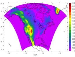
source of image from the NARCCAP website

Last week I posted twice on the BAMS article

Linda O. Mearns, Ray Arritt, Sébastien Biner, Melissa S. Bukovsky, Seth McGinnis, Stephan Sain, Daniel Caya, James Correia, Jr., Dave Flory, William Gutowski, Eugene S. Takle, Richard Jones, Ruby Leung, Wilfran Moufouma-Okia, Larry McDaniel, Ana M. B. Nunes, Yun Qian, John Roads, Lisa Sloan, Mark Snyder, 2012: The North American Regional Climate Change Assessment Program: Overview of Phase I Results. Bull. Amer.Met Soc. September issue. pp 1337-1362.

in

“The North American Regional Climate Change Assessment Program: Overview of Phase I Results” By Mearns Et Al 2012 – An Excellent Study But It Overstates Its Significance In The Multi-Decadal Prediction Of Climate

E-Mail To Linda Mearns On The 2012 BAMS Article On Dynamic Downscaling

I have had an e-mail response from Linda Mearns and she informed me that she is too busy to respond at this time. I have requested her permission to post her e-mails rejecting my request and will present if she gives me permission.

Quite frankly, I am disappointed as ignoring the issues that I summarized in my two posts is not the proper approach to advancing climate science.

I have succinctly summarized below what are the fundamental flaws in the use of regional downscaling with respect to multi-decadal climate predictions:

My Conclusions:

• The  Mearns et al 2012 BAMS paper with respect to type 2 downscaling it is an important new contribution.
• However, it’s application to climate change runs (type 4 downscaling) is inappropriate and misleading to the impacts and policy communities.

In order to refute the second conclusion, these following two questions must be answered in the affirmative:

1. Can a type 4 downscaling can be more accurate than a type 2 downscaling? Otherwise why not just start from regional reanalyses and assess what changes would have to occur in order to cause a negative impact to key resources, as we recommed in Pielke et al 2012.  Only then assess what is plausibly possible and how to mitigate/adapt to prevent a negative effect from occuring.

2. Have the regional climate models shown skill  in predicting changes over time in regional multi-decadal regional climate statistics?

My answer to both #1 and #2 are NO.

The  Mearns et al 2012 BAMS paper uses observed data, as processed through reanalyses, as lateral boundary conditions, and interior nudging when used. This provides a real world constraint on how much the regional model can diverge from reality. This is why we label it as type 2 downscaling.

The results of the Mearns et al 2012 BAMS paper cannot be used to justify providing changes in climate statistics to the impacts communities (i.e. through type 4 downscaling).

The actual ability of climate models to predict (in hindcast) EVEN the current climate is very limited. I documented this with a number of peer-reviewed papers in my posts

More CMIP5 Regional Model Shortcomings

CMIP5 Climate Model Runs – A Scientifically Flawed Approach.

The Hindcast Skill Of The CMIP Ensembles For The Surface Air Temperature Trend –  By Sakaguchi Et Al 2012.

Predicting “climate change” is  even more of a challenge. The climate models have shown NO skill at predicting CHANGES in regional climate statistics.

It may be convenient to ignore these issues in order to keep the grant and contract money flowing, but unless these fundamental flaws can be refuted, research money and time is being wastefully spent.

Comment On “A National Strategy for Advancing Climate Modeling” From The NRC

There is a new and, in my view, scientifically flawed report published by the National Research Council. The report is

 A National Strategy for Advancing Climate Modeling

I have a few comments on this report in my post today which document its failings. First, the overarching perspective of the authors of the NRC report is [highlight added]

As climate change has pushed climate patterns outside of historic norms, the need for detailed projections is growing across all sectors, including agriculture, insurance, and emergency preparedness planning. A National Strategy for Advancing Climate Modeling emphasizes the needs for climate models to evolve substantially in order to deliver climate projections at the scale and level of detail desired by decision makers, this report finds. Despite much recent progress in developing reliable climate models, there are still efficiencies to be gained across the large and diverse U.S. climate modeling community.

My Comment:

First, their statement that “….climate change has pushed climate patterns outside of historic norms” is quite a convoluted statement. Climate has always been changing. This insertion of “climate change” clearly is a misuse of the terminology “climate change” as I discussed in the post

The Need For Precise Definitions In Climate Science – The Misuse Of The Terminology “Climate Change”

Second, there are no reliable climate model predictions on multi-decadal time scale! This is clearly documented in the posts; e.g. see

Comments On The Nature Article “Afternoon Rain More Likely Over Drier Soils” By Taylor Et Al 2012 – More Rocking Of The IPCC Boat

More CMIP5 Regional Model Shortcomings

CMIP5 Climate Model Runs – A Scientifically Flawed Approach

The NRC Report also writes

Over the next several decades, climate change and its myriad consequences will be further unfolding and possibly accelerating, increasing the demand for climate information. Society will need to respond and adapt to impacts, such as sea level rise, a seasonally ice-free Arctic, and large-scale ecosystem changes. Historical records are no longer likely to be reliable predictors of future events; climate change will affect the likelihood and severity of extreme weather and climate events, which are a leading cause of economic and human losses with total losses in the hundreds of billions of dollars over the past few decades.

My Comment:

As I wrote earlier in this post, the multi-decadal climate model predictions have failed to skillfully predict not only changes in climate statistics over the past few decades, but cannot even accurately enough simulate the time averaged regional climates! Moreover, in terms of the comment that

“…climate change will affect the likelihood and severity of extreme weather and climate events, which are a leading cause of economic and human losses with total losses in the hundreds of billions of dollars over the past few decades.”

this is yet another example of where the BS meter is sounding off! See, for example, my son’s most recent discussion of this failing by the this climate community;

The IPCC sinks to a new low

The NRC report continues

Computer models that simulate the climate are an integral part of providing climate information, in particular for future changes in the climate. Overall, climate modeling has made enormous progress in the past several decades, but meeting the information needs of users will require further advances in the coming decades.

They also write that

Climate models skillfully reproduce important, global-to-continental-scale features of the present climate, including the simulated seasonal-mean surface air temperature (within 3°C of observed (IPCC, 2007c), compared to an annual cycle that can exceed 50°C in places), the simulated seasonal-mean precipitation (typical errors are 50% or less on regional scales of 1000 km or larger that are well resolved by these models [Pincus et al., 2008]), and representations of major climate features such as major ocean current systems like the Gulf Stream (IPCC, 2007c) or the swings in Pacific sea-surface temperature, winds and rainfall associated with El Niño (AchutaRao and Sperber, 2006; Neale et al., 2008). Climate modeling also delivers useful forecasts for some phenomena from a month to several seasons ahead, such as seasonal flood risks.

My Comment:  Actually “climate modeling” has made little progress in simulating regional climate on multi-decadal time scales, and no demonstrated evidence of being able to skillfully predict changes in the climate system. Indeed, the most robust work are the peer-reviewed papers that are in my posts (as I also listed earlier in this post)

Comments On The Nature Article “Afternoon Rain More Likely Over Drier Soils” By Taylor Et Al 2012 – More Rocking Of The IPCC Boat

More CMIP5 Regional Model Shortcomings

CMIP5 Climate Model Runs – A Scientifically Flawed Approach

which document the lack of skill in the models.

The report also defines “climate” as

Climate is conventionally defined as the long-term statistics of the weather (e.g., temperature, precipitation, and other meteorological conditions) that characteristically prevail in a particular region.

Readers of my weblog should know that this is an inappropriately narrow definition of climate. In the NRC report

National Research Council, 2005: Radiative forcing of climate change: Expanding the concept and addressing uncertainties. Committee on Radiative Forcing Effects on Climate Change, Climate Research Committee, Board on Atmospheric Sciences and Climate, Division on Earth and Life Studies, The National Academies Press, Washington, D.C., 208 pp.

(which the new NRC report conveniently ignored), climate is defined as

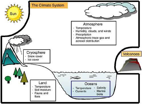
The system consisting of the atmosphere, hydrosphere, lithosphere, and  biosphere, determining the Earth’s climate as the result of mutual interactions  and responses to external influences (forcing). Physical, chemical, and  biological processes are involved in interactions among the components of the  climate system.

FIGURE 1-1 The climate system, consisting of the atmosphere, oceans, land, and cryosphere. Important state variables for each sphere of the climate system are listed in the boxes. For the purposes of this report, the Sun, volcanic emissions, and human-caused emissions of greenhouse gases and changes to the land surface are considered external to the climate system (from NRC, 2005)

This new NRC report “A National Strategy for Advancing Climate Modeling” misrepresents the capabilities of the climate models to simulate the climate system on multi-decadal time periods.

While I am in support of studies that assess the predictability skill of the models and to use them for monthly and seasonal predictions (which can be quickly tested against observations), seeking to advance climate modeling by claiming that more accurate multi-decadal regional forecasts can be made for policymakers and impact scientists and engineer with their proposed approach is, in my view, a dishonest communication to policymakers and to the public.

This need for advanced climate modeling should be promoted only and specifically with respect to assessing predictability on monthly,seasonal and longer time scales, not to making multi-decadal predictions for the impacts communties.

“The North American Regional Climate Change Assessment Program: Overview of Phase I Results” By Mearns Et Al 2012 – An Excellent Study But It Overstates Its Significance In The Multi-Decadal Prediction Of Climate

There is a new paper

Linda O. Mearns, Ray Arritt, Sébastien Biner, Melissa S. Bukovsky, Seth McGinnis, Stephan Sain, Daniel Caya, James Correia, Jr., Dave Flory, William Gutowski, Eugene S. Takle, Richard Jones, Ruby Leung, Wilfran Moufouma-Okia, Larry McDaniel, Ana M. B. Nunes, Yun Qian, John Roads, Lisa Sloan, Mark Snyder, 2012: The North American Regional Climate Change Assessment Program: Overview of Phase I Results. Bull. Amer.Met Soc. September issue. pp 1337-1362.

that provides further documentation of the level of skill of dynamic downscaling. It is a very important new contribution which will be widely cited. The participants in the North American Regional Climate Change Assessment Program  are listed here.

However, it significantly overstates the significance of its findings in terms of its application to the multi-decadal prediction of regional climate.

The paper is even highlighted on the cover of the September 2012 issue of BAMS, with the caption for the cover in the Table of Contents that reads

“Regional models are the foundation of research and services as planning for climate change requires more specific information than can be provided by global models. The North American Regional Climate Change Assessment Programs (Mearns et al., page 1337) evaluates uncertainties in using such models….”

Actually, as outlined below, the Mearns et al 2012 paper, while providing valuable new insight into one type of regional dynamic downscaling, is misrepresenting what these models can skillfully provide with respect to “climate change”.

The study uses observational data (from a Reanalysis) to drive the regional models. Using the classification we have introduced in our papers (see below), this is a type 2 dynamic downscaling study.

The Mearns et al 2012 paper only provides an upper bound of what is possible with respect to their goal to provide

“uncertainties in regional scale projections of future climate and produce high resolution climate change scenarios using multiple regional climate models (RCMs) nested within atmosphere ocean general circulation models (AOGCMs) forced with the A2 SRES scenario.”

The type of downscaling used in a study is a critically important point that needs to be emphasized when dynamic downscaling studies are presented.  Indeed, the new paper seeks to just replicate the current climate, NOT changes in climate statistics over the time period of the model runs.

It is even more challenging to skillfully predict CHANGES in regional climate which is what is required if the RCMs are to add any value for predicting climate in the coming decades.

The abstract and their short capsule reads [highlight added]

The North American Regional Climate Change Assessment Program is an international effort designed to investigate the uncertainties in regional scale projections of future climate and produce high resolution climate change scenarios using multiple regional climate models (RCMs) nested within atmosphere ocean general circulation models (AOGCMs) forced with the A2 SRES scenario, with a common domain covering the conterminous US, northern Mexico, and most of Canada. The program also includes an evaluation component (Phase I) wherein the participating RCMs, with a grid spacing 50 km, are nested within 25 years of NCEP/DOE global reanalysis II.

We provide an overview of our evaluations of the Phase I domain-wide simulations focusing on monthly and seasonal temperature and precipitation, as well as more detailed investigation of four sub-regions. We determine the overall quality of the simulations, comparing the model performances with each other as well as with other regional model evaluations over North America.  The metrics we use do differentiate among the models, but, as found in previous studies, it is not possible to determine a ‘best’ model among them. The ensemble average of the six models does not perform best for all measures, as has been reported in a number of global climate model studies. The subset ensemble of the 2 models using spectral nudging is more often successful for domain wide root mean square error (RMSE), especially for temperature. This evaluation phase of NARCCAP will inform later program elements concerning differentially weighting the models for use in producing robust regional probabilities of future climate change.

Capsule

This article presents overview results and comparisons with observations for temperature and precipitation from the six regional climate models used in NARCCAP driven by NCEP/DOE Reanalysis II (R2) boundary conditions for 1980 through 2004.

Using the types of dynamic downscaling that we present in the articles

Castro, C.L., R.A. Pielke Sr., and G. Leoncini, 2005: Dynamical downscaling:  Assessment of value retained and added using the Regional Atmospheric  Modeling System (RAMS). J. Geophys. Res. – Atmospheres, 110, No. D5, D05108,  doi:10.1029/2004JD004721.

Pielke Sr., R.A., and R.L. Wilby, 2012: Regional climate downscaling – what’s the point? Eos Forum,  93, No. 5, 52-53, doi:10.1029/2012EO050008.

the Mearns et al 2012 paper is a Type 2 downscaling. It provides an upper bound on the skill possible from Type 3 and Type 4 downscaling, since real world observations are used to constrain the model simulations (through the lateral boundary conditions, and from interior nudging if used).

These types of downscaling are defined in the Castro et al 2005 and Pielke and Wilby 2012 papers as

Type 1 downscaling is used for short-term, numerical weather prediction. In dynamic type 1 downscaling the regional model includes initial conditions from observations. In type 1 statistical downscaling the regression relationships are developed from observed data and the type 1 dynamic model predictions.

Type 2 dynamic downscaling refers to regional weather (or climate) simulations [e.g., Feser et al., 2011] in which the regional model’s initial atmospheric conditions are forgotten (i.e., the predictions do not depend on the specific initial conditions) but results still depend on the lateral boundary conditions from a global numerical weather prediction where initial observed atmospheric conditions are not yet forgotten or are from a global reanalysis. Type 2 statistical downscaling uses the regression relationships developed for type 1 statistical downscaling except that the input variables are from the type 2 weather (or climate) simulation. Downscaling from reanalysis products (type 2 downscaling) defines the maximum forecast skill that is achievable with type 3 and type 4 downscaling.

Type 3 dynamic downscaling takes lateral boundary conditions from a global model prediction forced by specified real world surface boundary conditions such as seasonal weather predictions based on observed sea surface temperatures, but the initial observed atmospheric conditions in the global model are forgotten [e.g., Castro et al., 2007]. Type 3 statistical downscaling uses the regression relationships developed for type 1 statistical downscaling except using the variables from the global model prediction forced by specified real-world surface boundary conditions.

Type 4 dynamic downscaling takes lateral boundary conditions from an Earth system model in which coupled interactions among the atmosphere, ocean, biosphere, and cryosphere are predicted [e.g., Solomon et al.,
2007]. Other than terrain, all other components of the climate system are calculated by the model except for human forcings, including greenhouse gas emissions scenarios, which are prescribed. Type 4 dynamic
downscaling is widely used to provide policy makers with impacts from climate decades into the future. Type 4 statistical downscaling uses transfer functions developed for the present climate, fed with large scale atmospheric information taken from Earth system models representing future climate conditions. It is assumed that statistical relationships between real-world surface observations and large-scale weather patterns will not change. Type 4 downscaling has practical value but with the very important caveat that it should be used for model sensitivity experiments and not as predictions [e.g., Pielke, 2002; Prudhomme et al., 2010].

Because real-world observational constraints diminish from type 1 to type 4 downscaling, uncertainty grows as more climate variables must be predicted by models, rather than obtained from observations.

The Mearns et al 2012 study concludes with the claim that

Our goal was to provide an overview of the relative performances of the six models both individually and as an ensemble with regard to temperature and precipitation. We have shown that all the models can simulate aspects of climate well, implying that they all can provide useful information about climate change. In particular, the results from phase I of NARCCAP will be used to establish uncertainty due to boundary conditions as well as final weighting of the models for the development of regional probabilities of climate change.

First, as documented in the article, the difference between  the models and the observations are actually significant. To claim that

“all the models can simulate aspects of climate well”

is not a robust claim.  What is meant by “well”?  The tables and figures in the article document significant biases in the temperatures and precipitation even for the current climate type 2 downscaling simulations.

Even more significantly, their type 2 downscaling study does NOT imply

“that they all can provide useful information about climate change”!

The  Mearns et al 2012 study did not look at the issue of their skill to predict CHANGES in climate statistics. For this they must examine type 4 downscaling skill, which they did not do.

In the context of the skill achieved with type 2 dynamic downscaling, this is an important, useful study.  However, to use the results of this type 2 downscaling study by Mearns et al 2012 to provide

“….final weighting of the models for the development of regional probabilities of climate change”

is a gross overstatement of what they accomplished. One cannot use type 2 downscaling to make claims about the accuracy of type 4 downscaling.

I am e-mailing the authors of the Mearns et al 2012 paper to request their response to my comments.  Each of them are well-respected colleagues and I will post their replies when they respond.

source of image

Comments On “The Shifting Probability Distribution Of Global Daytime And Night-Time Temperatures” By Donat and Alexander 2012 – A Not Ready For Prime Time Study

above figure from Caesar et al 2006

A new paper has appeared;

Donat, M. G. and L. V. Alexander (2012), The shifting probability distribution of global daytime and night-time temperatures, Geophys. Res. Lett., 39, L14707, doi:10.1029/2012GL052459.

The abstract reads [highlight added]

Using a global observational dataset of daily gridded maximum and minimum temperatures we investigate changes in the respective probability density functions of both variables using two 30-year periods; 1951–1980 and 1981–2010. The results indicate that the distributions of both daily maximum and minimum temperatures have significantly shifted towards higher values in the latter period compared to the earlier period in almost all regions, whereas changes in variance are spatially heterogeneous and mostly less significant. However asymmetry appears to have decreased but is altered in such a way that it has become skewed towards the hotter part of the distribution. Changes are greater for daily minimum (night-time) temperatures than for daily maximum (daytime) temperatures. As expected, these changes have had the greatest impact on the extremes of the distribution and we conclude that the distribution of global daily temperatures has indeed become “more extreme” since the middle of the 20th century.

This study, unfortunately, perpetuates the use of Global Historical Climate Reference Network surface temperature data as being a robust measure of surface temperature trends. The authors report that

 We use HadGHCND [Caesar et al., 2006], a global gridded data set of observed near-surface daily minimum (Tmin) and maximum (Tmax) temperatures from weather stations, available from 1951 and updated to 2010. For this study, we consider daily Tmax and Tmin anomalies calculated with respect to the 1961 to 1990 daily climatological average.

As described in the paper

Caesar, J., L. Alexander, and R. Vose (2006), Large-scale changes in observed daily maximum and minimum temperatures: Creation and analysis of a new gridded data set, J. Geophys. Res., 111, D05101, doi:10.1029/2005JD006280.

A gridded land-only data set representing near-surface observations of daily maximum and minimum temperatures (HadGHCND) has been created to allow analysis of recent changes in climate extremes and for the evaluation of climate model simulations. Using a global data set of quality-controlled station observations compiled by the U.S. National Climatic Data Center (NCDC), daily anomalies were created relative to the 1961–1990 reference period for each contributing station. An angular distance weighting technique was used to interpolate these observed anomalies onto a 2.5° latitude by 3.75° longitude grid over the period from January 1946 to December 2000. We have used the data set to examine regional trends in time-varying percentiles. Data over consecutive 5 year periods were used to calculate percentiles which allow us to see how the distributions of daily maximum and minimum temperature have changed over time. Changes during the winter and spring periods are larger than in the other seasons, particularly with respect to increasing temperatures at the lower end of the maximum and minimum temperature distributions. Regional differences suggest that it is not possible to infer distributional changes from changes in the mean alone.

The Donat and Alexander 2012 article concludes with the text

Using the data from this study we conclude that daily temperatures (both daytime and night-time) have indeed become “more extreme” and that these changes are related to shifts in multiple aspects of the daily temperature distribution other than just changes in the mean. However evidence is less conclusive as to whether it has become “more variable”.

The Donat and Alexander (2012) paper and the Caesar et al (2006) paper, however, both suffer in their ignoring issues that have been raised regarding the robustness of the data they are using for their analyses. They either ignored or are unaware of papers that show that the conclusions they give cannot be considered accurate unless they can show that the unresolved uncertainties  have either been corrected for, or shown not to affect their analyses. An overview of these issues is given in

Pielke Sr., R.A., C. Davey, D. Niyogi, S. Fall, J. Steinweg-Woods, K. Hubbard, X. Lin, M. Cai, Y.-K. Lim, H. Li, J. Nielsen-Gammon, K. Gallo, R. Hale, R. Mahmood, S. Foster, R.T. McNider, and P. Blanken, 2007: Unresolved issues with   the assessment of multi-decadal global land surface temperature trends. J. Geophys. Res., 112, D24S08, doi:10.1029/2006JD008229.

which the authors ignored in their study. The questions the authors did not examine before accepting the robustness of their analyses include:

1. The quality of station siting in the HadGHCND and whether this affects the extreme surface temperatures [Pielke et al 2002; Mahmood et al 2006; Fall et al 2011; Martinez et al 2012].

2. The effect of a concurrent change over time in the dew point temperatures at each HadGHCND location, which, if they are lower, could result in higher dry bulb temperatures [Davey et al 2006; Fall et al 2010; Peterson et al 2011 ]

3.  A bias in the siting of the HadGHCND observing sites for particular landscape types [Montandon et al 2011]

4. Small scale vegetation effects on maximum and minimum temperatures observed at HadGHCND sites [Hanamean et al 2003]

5. The uncertainty associated with each separate step in the HadGHCND homogenization method to develop grid area averages [Pielke 2005].

6. The warm bias that is expected to be in the HadGHCND with respect  to minimum temperatures [which would be expected to be even more pronounced with respect to extreme cold temperatures] [Klotzbach et al 2010,2011; McNider et al 2012].

As just one example from the above list, Mahmood et al 2006 finds that

…the difference in average extreme monthly minimum temperatures can be as high as 3.6 °C between nearby stations, largely owing to the differences in instrument exposures.’

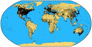
Note also in the figure at the top of this post, the poor spatial sampling for large portions of land.

The conclusion is that the HadGHCND data set is NOT sufficiently quality controlled, despite the assumption of the authors to the contrary. Ignoring peer reviewed papers that raise issues with their methodology does not follow the scientific  method.

The complete cite for these peer-reviewed papers that were ignored are listed below:

Davey, C.A., R.A. Pielke Sr., and K.P. Gallo, 2006: Differences between  near-surface equivalent temperature and temperature trends for the eastern  United States – Equivalent temperature as an alternative measure of heat  content. Global and Planetary Change, 54, 19–32.

Fall, S., N. Diffenbaugh, D. Niyogi, R.A. Pielke Sr., and G. Rochon, 2010: Temperature and equivalent temperature over the United States (1979 – 2005). Int. J. Climatol., DOI: 10.1002/joc.2094.

Fall, S., A. Watts, J. Nielsen-Gammon, E. Jones, D. Niyogi, J. Christy, and R.A. Pielke Sr., 2011: Analysis of the impacts of station exposure on the U.S. Historical Climatology Network temperatures and temperature trends. J. Geophys. Res.,  116, D14120, doi:10.1029/2010JD015146.Copyright (2011) American Geophysical Union.

Hanamean,  J.R. Jr., R.A. Pielke Sr., C.L. Castro, D.S. Ojima, B.C. Reed, and Z.  Gao, 2003: Vegetation impacts on maximum and minimum temperatures in northeast  Colorado. Meteorological Applications, 10, 203-215.

Klotzbach, P.J., R.A. Pielke Sr., R.A. Pielke Jr.,  J.R. Christy, and R.T. McNider, 2009: An alternative explanation for differential temperature trends at the  surface and in the lower troposphere. J. Geophys. Res., 114, D21102, doi:10.1029/2009JD011841.

Klotzbach, P.J., R.A. Pielke Sr., R.A. Pielke Jr.,  J.R. Christy, and R.T. McNider, 2010: Correction to: “An alternative explanation for differential temperature trends at the  surface and in the lower troposphere. J. Geophys. Res., 114, D21102, doi:10.1029/2009JD011841″, J. Geophys. Res.,  115, D1, doi:10.1029/2009JD013655

Mahmood, R., S. A. Foster, and D. Logan (2006a), The geoprofile metadata, exposure of instruments, and measurement bias in climatic record revisited, Int. J. Climatol., 26, 1091–1124.

Martinez, C.J., Maleski, J.J., Miller, M.F, 2012: Trends in precipitation and temperature in Florida, USA. Journal of Hydrology. volume 452-453, issue , year 2012, pp. 259 – 281

McNider, R.T., G.J. Steeneveld, B. Holtslag, R. Pielke Sr, S.   Mackaro, A. Pour Biazar, J.T. Walters, U.S. Nair, and J.R. Christy, 2012: Response and sensitivity of the nocturnal boundary layer over  land to added longwave radiative forcing. J. Geophys. Res., doi:10.1029/2012JD017578, in press.

Montandon, L.M., S. Fall, R.A. Pielke Sr., and D. Niyogi, 2011: Distribution of landscape types in the Global Historical Climatology Network. Earth Interactions, 15:6, doi: 10.1175/2010EI371

Peterson, T. C., K. M. Willett, and P. W. Thorne (2011), Observed changes in surface atmospheric energy over land, Geophys. Res. Lett., 38, L16707, doi:10.1029/2011GL048442

Pielke Sr., R.A., T. Stohlgren, L. Schell, W. Parton, N. Doesken, K. Redmond,  J. Moeny, T. McKee, and T.G.F. Kittel, 2002: Problems in evaluating regional  and local trends in temperature: An example from eastern Colorado, USA.  Int. J. Climatol., 22, 421-434.

Pielke Sr., Roger A., 2005: Public Comment on CCSP Report “Temperature Trends  in the Lower Atmosphere: Steps for Understanding and Reconciling Differences“. 88 pp including appendices.

The Donat and Alexander (2012) is particularly at fault in this neglect as most of the papers questioning the robustness of the GHCN type data sets were published well before their article was completed.  The conclusions of the Donat and Alexander study should not be considered as robust until they address the issues we raised in our papers.  

CMIP5 Climate Model Runs – A Scientifically Flawed Approach

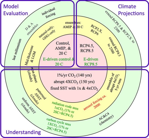
CMIP5 Climate model predictions for the coming decades is an integral part of the upcoming IPCC assessment.  The CMIP5 – Coupled Model Intercomparison Project Phase 5 is intended to

“to promote a new set of coordinated climate model experiments. These experiments  comprise the fifth phase of the Coupled Model Intercomparison Project (CMIP5).  CMIP5 will notably provide a multi-model context for 1) assessing the mechanisms  responsible for model differences in poorly understood feedbacks associated with  the carbon cycle and with clouds, 2) examining climate “predictability” and  exploring the ability of models to predict climate on decadal time scales, and,  more generally, 3) determining why similarly forced models produce a range of  responses.”

They report that

CMIP5 promotes a standard set of model simulations in order to:

• evaluate how realistic the models are in simulating the recent past,
• provide projections of future climate change on two time scales, near term (out to about 2035) and long term (out to 2100 and beyond), and
• understand some of the factors responsible for differences in model projections, including quantifying some key feedbacks such as those involving clouds and the carbon cycle

My post today is to summarize the lack of scientific value in those model predictions with respect to “evaluate how realistic the models are in simulating the recent past” and, thus their  use to project (predict) “future climate change on two time scales, near term (out to about 2035) and long term (out to 2100 and beyond.” My post brings together information from several recent posts.

The first requirement of the CMIP5 runs, before they should even be spending time and money on projections,  is that they must skillfully (and shown with quantitative analyses) to

•  replicate the statistics of the current climate,

and

• replicate the changes in climate statistics over this time period.

However, peer-reviewed studies that have quantitatively examined this issue using hindcast runs show large problems even with respect to current model statistics, much less their change over time. 

Examples of these studies include

1. Fyfe, J. C., W. J. Merryfield, V. Kharin, G. J. Boer, W.-S. Lee, and K. von Salzen (2011), Skillful predictions of decadal trends in global mean surface temperature, Geophys. Res. Lett.,38, L22801, doi:10.1029/2011GL049508

who concluded that

”….for longer term decadal hindcasts a linear trend correction may be required if the model does not reproduce long-term trends. For this reason, we correct for systematic long-term trend biases.”

2. Xu, Zhongfeng and Zong-Liang Yang, 2012: An improved dynamical downscaling method with GCM bias corrections and its validation with 30 years of climate simulations. Journal of Climate 2012 doi: http://dx.doi.org/10.1175/JCLI-D-12-00005.1

who find that without tuning from real world observations, the model predictions are in significant error. For example, they found that

”…the traditional dynamic downscaling (TDD) [i.e. without tuning) overestimates precipitation by 0.5-1.5 mm d-1…..The 2-year return level of summer daily maximum temperature simulated by the TDD is underestimated by 2-6°C over the central United States-Canada region.”

3. van Oldenborgh, G.J., F.J. Doblas-Reyes, B. Wouters, W. Hazeleger (2012): Decadal prediction skill in a multi-model ensemble. Clim.Dyn. doi:10.1007/s00382-012-1313-4

who report quite limited predictive skill in two regions of the oceans on the decadal time period, but no regional skill elsewhere, when they conclude that

“A 4-model 12-member ensemble of 10-yr hindcasts has been analysed for skill in SST, 2m temperature and precipitation. The main source of skill in temperature is the trend, which is primarily forced by greenhouse gases and aerosols. This trend contributes almost everywhere to the skill. Variation in the global mean temperature around the trend do not have any skill beyond the first year. However, regionally there appears to be skill beyond the trend in the two areas of well-known low-frequency variability: SST in parts of the North Atlantic and Pacific Oceans is predicted better than persistence. A comparison with the CMIP3 ensemble shows that the skill in the northern North Atlantic and eastern Pacific is most likely due to the initialisation, whereas the skill in the subtropical North Atlantic and western North Pacific are probably due to the forcing.”

4. Anagnostopoulos, G. G., Koutsoyiannis, D., Christofides, A., Efstratiadis, A. & Mamassis, N. (2010) A comparison of local and aggregated climate model outputs with observed data. Hydrol. Sci. J. 55(7), 1094–1110

who report that

“…. local projections do not correlate well with observed measurements. Furthermore, we found that the correlation at a large spatial scale, i.e. the contiguous USA, is worse than at the local scale.”

5. Stephens, G. L., T. L’Ecuyer, R. Forbes, A. Gettlemen, J.‐C. Golaz, A. Bodas‐Salcedo, K. Suzuki, P. Gabriel, and J. Haynes (2010), Dreary state of precipitation in global models, J. Geophys. Res., 115, D24211, doi:10.1029/2010JD014532.

who wrote

“models produce precipitation approximately twice as often as that observed and make rainfall far too lightly…..The differences in the character of model precipitation are systemic and have a number of important implications for modeling the coupled Earth system …….little skill in precipitation [is] calculated at individual grid points, and thus applications involving downscaling of grid point precipitation to yet even finer‐scale resolution has little foundation and relevance to the real Earth system.”

6. Sun, Z., J. Liu, X. Zeng, and H. Liang (2012), Parameterization of instantaneous global horizontal irradiance at the surface. Part II: Cloudy-sky component, J. Geophys. Res., doi:10.1029/2012JD017557, in press.

who report that

“Radiation calculations in global numerical weather prediction (NWP) and climate models are usually performed in 3-hourly time intervals in order to reduce the computational cost. This treatment can lead to an incorrect Global Horizontal Irradiance (GHI) at the Earth’s surface, which could be one of the error sources in modelled convection and precipitation. …… An important application of the scheme is in global climate models. The radiation sampling error due to infrequent radiation calculations is investigated using the this scheme and ARM observations. It is found that these errors are very large, exceeding 800 W m-2 at many non-radiation time steps due to ignoring the effects of clouds….”

7. Ronald van Haren, Geert Jan van Oldenborgh, Geert Lenderink, Matthew Collins and Wilco Hazeleger, 2012: SST and circulation trend biases cause an underestimation of European precipitation trends Climate Dynamics 2012, DOI: 10.1007/s00382-012-1401-5

who report that

“To conclude, modeled atmospheric circulation and SST trends over the past century are significantly different from the observed ones. These mismatches are responsible for a large part of the misrepresentation of precipitation trends in climate models. The causes of the large trends in atmospheric circulation and summer SST are not known.”

Even the most basic of climate model predictions that global average water vapor is increasing (and thus would amplify the radiative warming from added CO2) is in question; see

Vonder Haar, T. H., J. Bytheway, and J. M. Forsythe (2012), Weather and climate analyses using improved global water vapor observations, Geophys. Res. Lett.,doi:10.1029/2012GL052094, in press.

There is an important summary of the limitations in multi-decadal regional climate predictions in

Kundzewicz, Z. W., and E.Z. Stakhiv (2010) Are climate models “ready for prime time” in water resources managementapplications, or is more research needed? Editorial. Hydrol. Sci. J. 55(7), 1085–1089.

who conclude that

“Simply put, the current suite of climate models were not developed to provide the level of accuracy required for adaptation-type analysis.”

These studies, and I am certain more will follow, show that the multi-decadal climate models are not even skillfully simulating current climate statistics, as are needed by the impacts communities, much less CHANGES in climate statistics.  At some point, this waste of money to make regional climate predictions decades from now is going to be widely recognized.

source of image

An Example Of Media Hype By John Vidal In The Guardian

There is a news article in the Guardian on July 4 2012 by John Vidal titled

As the climate changes, extreme weather isn’t that extreme any more

This is a good example of the type of reporting that my son talked about in his post

A Handy Bullshit Button on Disasters and Climate Change

In his post he writes

Anytime that you read claims that invoke disasters loss trends as an indication of human-caused climate change, including  the currently popular “billion dollar disasters” meme, you can simply call “bullshit” and point to the IPCC SREX report.

The Guardian article includes the remarkable statement that [highlight added]

There’s always been freak weather, but climatologists increasingly think these events are becoming less unusual. Instead of taking place every 10 or 20 years, they are happening every two or three. This, they are beginning to say, is the new normal, a taste of the future as the planet warms.

Apparently, it is okay to “think these events are becoming less unusual” to make the statement true.  However, the reality is not definitive with respect to extremes.  We examined this in our paper with respect to the European 2003 heat wave

Chase, T.N., K. Wolter, R.A. Pielke Sr., and Ichtiaque Rasool, 2006: Was  the 2003 European summer heat wave unusual in a global context? Geophys.  Res. Lett.,  33, L23709, doi:10.1029/2006GL027470.

Chase, T.N., K. Wolter, R.A. Pielke Sr., and Ichtiaque Rasool, 2008: Reply to comment by W.M. Connolley on ‘‘Was the 2003 European summer heat wave unusual in a global context?’’Geophys.  Res. Lett., 35, L02704, doi:10.1029/2007GL031574.

and our conclusion was confirmed in

Connolley  W.M. 2008: Comment on  “Was  the 2003 European summer heat wave unusual in a global context?” by Thomas N. Chase et al. Geophys.  Res. Lett., 35, L02703, doi:10.1029/2007GL031171.

It is only with robust scientific assessments will the answer be obtained as to whether the frequency of extreme weather has changed.

The last sentence of the Guardian article shows that this “news” article is really an op-ed. John Vidale writes

This is a most dangerous period. We still have a very good chance of avoiding the worst of climate change but the collective will to try to do anything appears to be weakening and confidence in politicians is at rock bottom. Unless the climate of opinion changes, the present economic storms may seem as nothing.

The current distribution of cool and warm extreme events certainly warrants explanation. As I have posted in

Perspective On The Hot and Dry Continental USA For 2012 Based On The Research Of Judy Curry and Of McCabe Et Al 2004

it is the spatial arrangement of atmospheric and ocean circulation features that matter much more than a global average surface temperature anomaly. As shown in the University of Alabama at Huntsville data for  May 2012 (see), for example, the lower tropospheric temperature anomaly is just +0.29 C above the 30 year average.  As shown by Bob Tisdale (see) the global averaged sea surface temperature anomaly for June (from the Reynolds OI.v.2 SST) is only +0.191 C above its long-term average.

While humans certainly are influencing the climate system, “global warming” (whether caused in part, or even all, by humans) seems to be a rather small component. As we wrote in one of my first weblog posts in 2005

What is the Importance to Climate of Heterogeneous Spatial Trends in Tropospheric Temperatures?

“…regional diabatic heating produces temperature increases or decreases in the layer-averaged regional troposphere. This necessarily alters the regional pressure fields and thus the wind pattern. This pressure and wind pattern than affects the pressure and wind patterns at large distances from the region of the forcing which we refer to as teleconnections.”

It is these regional circulation features that are the reason for the current heat wave in large parts of the USA and the  “lost summer” of 2012 in Europe.  John Vidale, in his Guardian news article, ignores presenting evidence that human activity is the reason for the current spatial pattern of atmospheric and ocean circulations, and how they would be different without human effects.  He has grossly oversimplified how the real climate system behaves.

source of image

Comment On Seth Borenstein AP News Article “This US Summer Is ‘What Global Warming Looks Like'”

Image of drought in July 1936 from NOAA NCDC

There are at least two  excellent (as usual) posts [that I have seen so far] on Seth Borenstein AP news article

This US summer is ‘what global warming looks like’

in Judy Curry’s post

What global warming looks like (?)

and Anthony Watt’s post

The Kevin Trenberth / Seth Borenstein aided fact free folly on the USA heat wave

I have posted on the current extreme weather (and placed it in context) in my posts

Perspective On The Hot and Dry Continental USA For 2012 Based On The Research Of Judy Curry and Of McCabe Et Al 2004

The Great Fire Of 1910 Places The Current 2012 Fire Season In Perspective

Guest Post On “Fire Suppression Policy, Weather And Western Wildland Fire Trends: An Empirical Analysis” By Johnston and Klick 2012

The news report contains the same type of quotes from the same individuals that are usually interviewed when we have extreme weather. Seth should know better by now, and I can only assume he really does want to present a biased news article.

Judy Curry, who was interviewed by Seth (but was ignored in the article) posted her answers to his questions, and I have reproduced below. I am completely in agreement with her responses.

JC comments

I received an email from Borenstein yesterday, asking me 6 questions, to which I responded.  My responses were not included in the article.  Here are the questions and my responses:

SB: Can you characterize what’s going in the US in terms of a future/present under climate change? Is it fair to say this is what other scientists been talking about?

JC:  As global average temperature increases, you can expect periodically there to be somewhere on the globe where weather patterns conspire to produce heat waves that are unusual relative to previous heat waves. However, there have been very few events say in the past 20 years or so that have been unprecedented say since 1900.

SB:  Is this what scientists behind the SREX meant? Why?

JC:  In the SREX report, they did not find any unambiguous observational evidence to attribute any extreme events to greenhouse warming, but then went on to speculate (based upon model simulations) what future warming would look like. These speculations are fairly general, and have little regional specificity since the models are currently incapable of simulating regional climate variability.

SB:  This seems to be only US? Is it fair to make a big deal, since this is small scale and variability and is only US? However in past years, especially in late 1990s and early 2000s, the US seemed to be less affected? So what should we make of it?

JC:  Right now, this is only the U.S. Recall, 2010 saw the big heat wave in Russia (whereas in the U.S. we had a relatively moderate summer, except for Texas). Note, the southern hemisphere (notably Australia and New Zealand) is having an unusually cold winter.

SB:  IS there any extreme that’s a function of climate change that we’re missing this summer? If so, what?

JC:  Not that I know of.

SB:  So might call this an I told you so moment? What do you think?

JC:  Extreme events definitely focus people’s attention on climate change, and a local heat wave can certainly do this. By the same token, the cold snow winter of 2010/2011 made people question greenhouse warming. Also, think Hurricane Katrina, which was another focusing event in the US for global warming

SB:  What about natural variability? Are other scientists just making too much of what is normal weather variability?

JC: We saw these kinds of heat waves in the 1930′s, and those were definitely not caused by greenhouse gases. Weather variability changes on multidecadal time scales, associated with the large ocean oscillations. I don’t think that what we are seeing this summer is outside the range of natural variability for the past century. In terms of heat waves, particularly in cities, urbanization can also contribute to the warming (the so-called urban heat island effect).

To add to Judy’s insightful answer, I have posted below an extract from Wikipedia on the 1936 heat wave over the USA [highlight added]

The heat wave started in late June, when temperatures across the US exceeded 100 °F (38 °C). The Midwest experienced some of the highest June temperatures on record. Drought conditions worsened. In the Northeast, temperatures climbed to the mid 90s °F (around 35 °C). The South and West started to heat up also, and also experienced drought. The heat wave began to extend into Canada. Moderate to extreme drought covered the entire continent. The dry and exposed soil contributed directly to the heat as happens normally in desert areas as the extreme heat entered the air by radiation and direct contact. Reports at the time and explored in the definitive works on the Dust Bowl told of soil temperatures reaching in excess of 200 °F (93 °C) at the four inch/10 cm level in regions of the Dust Bowl; such soil temperatures were sufficient to sterilize the soil by killing nitrogen-fixing bacteria and other microbes, delivering the final blow in the declining fertility of that soil which had not already blown away.[dubious – discuss]

July was the peak month, in which temperatures reached all-time record levels—many of which still stand as of 2010. In Steele, North Dakota, temperatures reached 121 °F (49 °C), which remains North Dakota’s record. In Ohio, temperatures reached 110 °F (43 °C), which nearly tied the previous record set in 1934. The states of Texas, Oklahoma, Kansas, Arkansas, Minnesota, Michigan, North Dakota, South Dakota, Pennsylvania, Louisiana, Nebraska, Wisconsin, West Virginia, and New Jersey also experienced record high temperatures. The provinces of Ontario and Manitoba set still-standing record highs above 110 °F (43 °C). Chicago Midway airport recorded 100 °F (38 °C) or higher temperatures on 12 consecutive days from July 6–17, 1936. Later that summer in downstate Illinois, at Mount Vernon the temperature surpassed 100 °F (38 °C) for 18 days running from August 12–29, 1936.[1]

Some stations in the American Midwest reported minimum temperatures at or above 90 °F (32 °C) such as 91 °F (33 °C) at Lincoln, Nebraska on July 25, 1936; the next and most recent time this is known to have happened is a handful of 90 °F (32 °C) minimums during a similar heat wave in late June 1988 but far less intense than that of 1936.

August was the warmest month on record for five states. Many experienced long stretches of daily maximum temperatures 100 °F (38 °C) or warmer. Drought conditions worsened in some locations. Some states were only slightly above average.

The heat wave and drought largely ended in September, though many states were still drier and warmer than average. Many farmers’ summer harvests were destroyed. Grounds and lawns remained parched. Annual temperatures returned to normal in the fall.

Seth Borenstein, by not including the diversity of perspectives on the current extreme weather, is not objectively reporting on this newsworthy weather event. The current heat and drought are not unprecedented. Moreover, the message should be that we need to prepare for such droughts, regardless of the role humans have in possibly altering their intensity and extent. If we look at the recent paleo-record; e.g. see

New Paper “A Long-Term Perspective On A Modern Drought In The American Southeast” By Pederson Et Al 2012

The Value Of Paleoclimate Records In Assessing Vulnerability to Drought: A New Paper Meko et al 2008

we see much more serious and longer lasting droughts than even occurred in the 1930s.  See also

Pielke, R.A. Sr., 2004: Discussion Forum: A broader perspective on climate change is needed. IGBP Newsletter, 59, 16-19.

Seth Borenstein’s article should have been written with the title “This US Summer Is ‘What Drought Looks Like’ and than reported on ways to reduce societal and environmental vulnerability to these events. Instead, he is further recognized as a reporter with an agenda who selects scientists to interview whose views (with just one exception) support his biases on the climate issue.

The Contrast Between The NOAA NCDC and NASA NEO Images Of Land Surface Temperature Anomalies – Further Evidence Of The NOAA Warm Bias

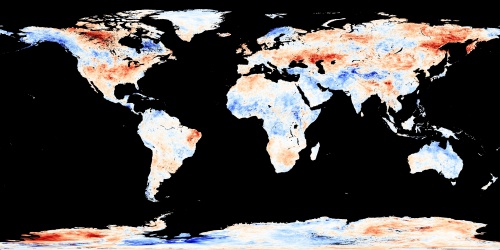
Image from NASA Earth Observations (NEO) for the May 1 to May 31 2012 surface temperature anomalies

Earlier this week, I posted

Comments On Missing Context Information In NOAA’s Report On The Large Positive Land Surface Temperature Anomalies in May 2012

and pointed out a number of problems with the NOAA NCDC data analysis based on the GHCN data, including its warm bias.  Today, I present at the top of this post the May 2012 surface temperature anomaly analysis from NASA’s Earth Observations program.

As written on the NASA’s Earth Observations program website

Land surface temperature is how hot or cold the ground feels to the touch. An anomaly is when something is different from average. These maps show where Earth’s surface was warmer or cooler in the daytime than the average temperatures for the same week or month from 2001-2010. So, a land surface temperature anomaly map for May 2002 shows how that month’s average temperature was different from the average temperature for all Mays between 2001 and 2010.

These maps show land surface temperature anomalies for a given day, week, or month compared to the average conditions during that period between 2000-2008. Places that are warmer than average are red, places that were near-normal are white, and places that are cooler than average are blue. Black means there is no data.

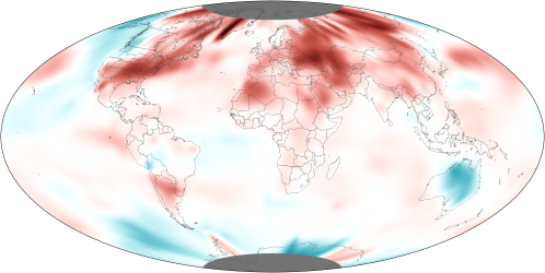
As a reminder, below is the NOAA NCDC analysis for May 2012

It does not take a quantitative analysis to see regions of large differences, such as the cool anomalies in the NASA data in Africa, Scandinavia, and elsewhere. While they are not measuring the same temperatures, the anomalies should be quite similar [For the GHCN, NOAA NCDC uses air temperature measurements which are supposed to be 2m above the ground; they also use the mean temperature anomalies which are computed using maximum and minimum temperatures].

The areal coverage of the temperature anomalies, however, are not the same. The NOAA analysis shows much larger areas of warmer than average surface temperatures than seen in the NASA NEO analysis.

This is yet another documentation of the warm bias in the NOAA NCDC analyses which they use for their press releases on how warm the climate has become. Now that the American Meteorological Society has published its statement “Freedom of Scientific Expression” where they wrote

it is incumbent upon scientists to  communicate their findings in ways that portray their results and the results  of others, objectively, professionally, and without sensationalizing or  politicizing the associated impacts

lets see if Tom Karl, Tom Peterson and others at NCDC finally start to present the diversity of information (and the uncertainties) of what the surface temperature anomalies actually are telling us.

Comments On Missing Context Information In NOAA’s Report On The Large Positive Land Surface Temperature Anomalies in May 2012

The above figure shows a picture of warmer than average land surface temperatures almost everywhere. This image is from the NOAA report

Global land temperature in May 2012 is warmest on record

It is created, as described in the NOAA article, as a

NOAA map by Dan Pisut, based on Global Historical Climatology Network data from the National Climatic Data Center (NCDC). Caption by Susan Osborne, NCDC. Reviewed by Jessica Blunden, NCDC Climate Monitoring Branch.

However, while it certainly shows a very warm period at the surface, there are caveats in this analysis:

1. The data is not as dense or as uniform as presented in this figure; eg. see the figure below

source of image from climanova.wordpress.com

Large land areas are dependent on just a few or no surface observing sites.

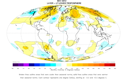
2. While the lower tropospheric data shows a very warm May, it is not as anomalous as at the surface as diagnosed by the Global Historical Climatology Network. The spatial map of lower tropospheric temperatures for May 2012 is shown below

In this data, May 2012 has a global composite lower tropospheric temperature anomaly of +0.29 C (about 0.52 degrees Fahrenheit) above 30-year average for May. The NOAA plot above has a global composite of “more than 1°F above the 20th century average” according to the NOAA article.

3. This divergence between the surface temperature analysis and the lower tropospheric temperature analyses is further demonstration of the divergence between these two data sets as we reported on in

Klotzbach, P.J., R.A. Pielke Sr., R.A. Pielke Jr.,  J.R. Christy, and R.T. McNider, 2009: An alternative explanation for differential temperature trends at the  surface and in the lower troposphere. J. Geophys. Res., 114, D21102, doi:10.1029/2009JD011841.

Klotzbach, P.J., R.A. Pielke Sr., R.A. Pielke Jr.,  J.R. Christy, and R.T. McNider, 2010: Correction to: “An alternative explanation for differential temperature trends at the  surface and in the lower troposphere. J. Geophys. Res., 114, D21102, doi:10.1029/2009JD011841″, J. Geophys. Res.,  115, D1, doi:10.1029/2009JD013655.

In a paper in press, which I will post on soon, we show that there is a warm bias in the minimum land temperatures which are used to create the land temperature anomalies that are presented in the NOAA GHCN figure.

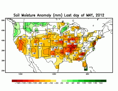
4. The reason that the surface temperature anomaly is so much larger than higher in the troposphere (for the mid tropospheric anomalies, see NOAA CPC) appears to be related to the exceptionally dry soil conditions across much of the USA, as shown for May 2012 below from NOAA’s Climate Prediction Center.

As we discussed in our paper

Pielke, R.A. Sr., K. Wolter, O. Bliss, N. Doesken, and B. McNoldy, 2007:  The July 2005 Denver heat wave: How unusual was it? Nat. Wea. Dig.,  31, 24-35

when the effect of temperature and humidity are combined (moist enthalpy), this provides a markedly different perspective, than using temperature alone. In the July 2005 heat wave discussed in the above paper, the Denver heat wave was less extreme using this combined metric, due to very low humidity accompanying the event. This is also a major factor in the current heat wave.

The mid-tropospheric anomalies for the past 15 days from the University of Albany is presented below which further documents that the tropospheric anomalies over most of the land areas, including the USA, are much less than at the surface.

Thus, the conclusion regarding the NOAA GHCN analysis and the news report based on it is neglects to also report that the same magnitude of anomaly does not exist higher in the troposphere.  Thus the reason for the warm surface temperatures needs further explanation.  In this post I pose that the larger surface temperature anomaly is due to

• the concurrent occurrence of dry soils results in a larger fraction of solar radiation being converted to sensible heat (i.e. measured by the dry bulb temperature) rather than into latent heat fluxes (evaporation and transpiration). This results in a higher dry bulb temperature than it otherwise would be. It is correct, however, that, based on the lower tropospheric temperature analyses, that most land areas appear to be warmer than average for May, but the surface anomalies are significantly larger.
• the surface data also, however, contains an effect of local microclimate changes that results in a local elevation of the nighttime minimum temperatures from what this temperature would have been in the past. The grid-averaging and homogenization algorithms used by NCDC smear this warm effect (which may be applicable only to a very small location) over large areas. This will be discussed further when our new paper is reported on.  This is an issue in addition to the siting quality question in the study led by Anthony Watts that we reported on it Fall et al 2011.
• the use of the GHCN as a diagnostic for the magnitude of global warming has a number of major complications including the neglect of concurrent surface anomalies in water vapor, siting quality issues, and local microclimate effects at GHCN sites which are inappropriately extrapolated over large regions.