Excellent New Paper “The Climate Is Not What You Expect” By Lovejoy and Schertzer 2012

I was alerted to an informative new paper on the issue of what is climate [h/t to Philip Richens]. The paper highlights the nonstationarity of climate as we presented in the papers

Pielke, R.A., 1998: Climate prediction as an initial value problem. Bull.  Amer. Meteor. Soc., 79, 2743-2746.

As I wrote in that paper

“weather prediction is a subset of climate prediction and that both are, therefore, initial value problems in the context of nonlinear geophysical flow.’

“…..longer-term feedback and physical processes must be included. This makes climate prediction a much more difficult problem than weather prediction”.

As we wrote in

Rial, J., R.A. Pielke Sr., M. Beniston, M. Claussen, J. Canadell, P. Cox,  H. Held, N. de Noblet-Ducoudre, R. Prinn, J. Reynolds, and J.D. Salas,  2004: Nonlinearities, feedbacks and critical thresholds within the Earth’s  climate system. Climatic Change, 65, 11-38.

The Earth’s climate system is highly nonlinear: inputs and outputs are not proportional, change is often episodic and abrupt, rather than slow and gradual, and multiple equilibria are the norm.

The new paper on this subject is

“The Climate Is Not What You Expect” By S. Lovejoy and D. Schertzer 2012 [submitted]

The abstract reads [highlight added]

Prevailing definitions of climate are not much different from “the climate is what you expect, the weather is what you get”. Using a variety of sources including reanalyses and paleo data, and aided by notions and analysis techniques from Nonlinear Geophysics, we argue that this dictum is fundamentally wrong. In addition to the weather and climate, there is a qualitatively distinct intermediate regime extending over a factor of ≈ 1000 in scale. For example, mean temperature fluctuations increase up to about 5 K at 10 days (the lifetime of planetary structures), then decrease to about 0.2 K at 30 years, and then increase again to about 5 K at glacial-interglacial scales. Both deterministic GCM’s with fixed forcings (“control runs”) and stochastic turbulence-based models reproduce the first two regimes, but not the third. The middle regime is thus a kind of low frequency “macroweather” not “high frequency climate”. Regimes whose fluctuations increase with scale appear unstable whereas regimes where they decrease appear stable. If we average macroweather states over periods ≈ 30 years, the results thus have low variability. In this sense, macroweather is what you expect.

We can use the critical duration of ≈ 30 years to define (fluctuating) “climate states”. As we move to even lower frequencies, these states increasingly fluctuate – appearing unstable so that the climate is not what you expect. The same methodology allows us to categorize climate forcings according to whether their fluctuations decrease or increase with scale and this has important implications for GCM’s and for climate change and climate predictions.

The conclusion reads

Contrary to [Bryson, 1997], we have argued that the climate is not accurately viewed as the statistics of fundamentally fast weather dynamics that are constrained by quasi fixed boundary conditions. The empirically substantiated picture is rather one of unstable (high frequency) weather processes tending – at scales beyond 10 days or so and primarily due to the quenching of spatial degrees of freedom – to quasi stable (intermediate frequency, low variability) macroweather processes. Climate processes only emerge from macroweather at even lower frequencies, and this thanks to new slow  internal climate processes coupled with external forcings. Their synergy yields fluctuations that on average again grow with scale and become dominant typically on time scales of 10 – 30 years up to ≈ 100 kyrs.

Looked at another way, if the climate really was what you expected, then – since one expects averages – predicting the climate would be a relatively simple matter. On the contrary, we have argued that from the stochastic point of view – and notwithstanding the vastly different time scales – that predicting natural climate change is very much like predicting the weather. This is because the climate at any time or place is the consequence of climate changes that are (qualitatively and quantitatively) unexpected in very much the same way that the weather is unexpected.

There are a series of informative comments on this paper by Judy Curry, Philip Richens, Shaun Lovejoy and others on the weblog All Models are Wrong post

Limitless Possibilities

In the insightful comment by Shaun Lovejoy on that weblog, he does write on one issue that I disagree with. Shaun writes

“….deterministic models (GCM’s) reproduce only weather and macroweather statistics (they do this quite well)”.

I agree on weather, but not on macroweather. Macroweather prediction has shown little, if any skill ; e.g. see the papers listed in my post

Kevin Trenberth Was Correct – “We Do Not Have Reliable Or Regional Predictions Of Climate”

As reported in that post, the papers reported on below document the failure to so far skillfully predict macroweather [what I refer to as climate, based on the definitions of  climate as a system in NRC 2005].

1. Fyfe, J. C., W. J. Merryfield, V. Kharin, G. J. Boer, W.-S. Lee, and K. von Salzen (2011), Skillful predictions of decadal trends in global mean surface temperature,  Geophys. Res. Lett.,38, L22801, doi:10.1029/2011GL049508

who concluded that

”….for longer term decadal hindcasts a linear trend correction may be required if the model does not reproduce long-term trends. For this reason, we correct for systematic long-term trend biases.”

2. Xu, Zhongfeng and Zong-Liang Yang, 2012: An improved dynamical downscaling method with GCM bias corrections and its validation with 30 years of climate simulations. Journal of Climate 2012 doi: http://dx.doi.org/10.1175/JCLI-D-12-00005.1

who find that without tuning from real world observations, the model predictions are in significant error. For example, they found that

”…the traditional dynamic downscaling (TDD) [i.e. without tuning) overestimates precipitation by 0.5-1.5 mm d-1…..The 2-year return level of summer daily maximum temperature simulated by the TDD is underestimated by 2-6°C over the central United States-Canada region.”

3. van Oldenborgh, G.J., F.J. Doblas-Reyes, B. Wouters, W. Hazeleger (2012): Decadal prediction skill in a multi-model ensemble. Clim.Dyn. doi:10.1007/s00382-012-1313-4

who report quite limited predictive skill in two regions of the oceans on the decadal time period, but no regional skill elsewhere,  when they conclude that

“A 4-model 12-member ensemble of 10-yr hindcasts has been analysed for skill in SST, 2m temperature and precipitation. The main source of skill in temperature is the trend, which is primarily forced by greenhouse gases and aerosols. This trend contributes almost everywhere to the skill. Variation in the global mean temperature around the trend do not have any skill beyond the first year. However, regionally there appears to be skill beyond the trend in the two areas of well-known low-frequency variability: SST in parts of the North Atlantic and Pacific Oceans is predicted better than persistence. A comparison with the CMIP3 ensemble shows that the skill in the northern North Atlantic and eastern Pacific is most likely due to the initialisation, whereas the skill in the subtropical North Atlantic and western North Pacific are probably due to the forcing.”

4. Anagnostopoulos, G. G., Koutsoyiannis, D., Christofides, A., Efstratiadis, A. & Mamassis, N. (2010) A comparison of local and aggregated climate model outputs with observed data. Hydrol. Sci. J. 55(7), 1094–1110

who report that

“…. local projections do not correlate well with observed measurements. Furthermore, we found that the correlation at a large spatial scale, i.e. the contiguous USA, is worse than at the local scale.”

5.  Stephens, G. L., T. L’Ecuyer, R. Forbes, A. Gettlemen, J.‐C. Golaz, A. Bodas‐Salcedo, K. Suzuki, P. Gabriel, and J. Haynes (2010), Dreary state of precipitation in global models, J. Geophys. Res., 115, D24211, doi:10.1029/2010JD014532.

who wrote

“models produce precipitation approximately twice as often as that observed and make rainfall far too lightly…..The differences in the character of model precipitation are systemic and have a number of important implications for modeling the coupled Earth system …….little skill in precipitation [is] calculated at individual grid points, and thus applications involving downscaling of grid point precipitation to yet even finer‐scale resolution has little foundation and relevance to the real Earth system.”

In response to my request to post on Shaun’s paper, he and I had a valuable e-mail interaction which I am posting below with his permission.

My initial query with Shaun’s reply embedded (as in the e-mail)

Hi Shaun

I was alerted by Philip to your excellent new paper

http://www.physics.mcgill.ca/~gang/eprints/eprintLovejoy/esubmissions/climate.not.26.6.12.pdf

Do I have your permission to post on my weblog an announcement about it along with the abstract and the conclusion? I would link to your pdf above where readers can obtain the full paper.

I have thought along the same lines as you have; e.g. see

Pielke, R.A., 1998: Climate prediction as an initial value problem. Bull. Amer. Meteor. Soc., 79, 2743-2746. https://pielkeclimatesci.files.wordpress.com/2009/10/r-210.pdf

Rial, J., R.A. Pielke Sr., M. Beniston, M. Claussen, J. Canadell, P. Cox, H. Held, N. de Noblet-Ducoudre, R. Prinn, J. Reynolds, and J.D. Salas, 2004: Nonlinearities, feedbacks and critical thresholds within the Earth’s climate system. Climatic Change, 65, 11-38. https://pielkeclimatesci.files.wordpress.com/2009/10/r-260.pdf

Pielke, R.A. and X. Zeng, 1994: Long-term variability of climate. J. Atmos. Sci., 51, 155-159. https://pielkeclimatesci.files.wordpress.com/2009/09/r-120.pdf

Pielke Sr., R.A., R. Wilby, D. Niyogi, F. Hossain, K. Dairuku, J. Adegoke, G. Kallos, T. Seastedt, and K. Suding, 2012: Dealing with complexity and extreme events using a bottom-up, resource-based vulnerability perspective. AGU Monograph on Complexity and Extreme Events in Geosciences, in press. https://pielkeclimatesci.files.wordpress.com/2011/05/r-365.pdf

If you approve, I plan to post for tomorrow.

Best Regards

Roger

P.S. Hi again Shaun

I was just alerted by Philip of your post on Tamsin Edward’s blog

http://allmodelsarewrong.com/limitless-possibilities/#comment-1397

and that of Judy Curry

http://allmodelsarewrong.com/limitless-possibilities/#comment-1238

and

http://allmodelsarewrong.com/limitless-possibilities/#comment-1257

On your comments, there is one I disagree with. You wrote

“….deterministic models (GCM’s) reproduce only weather and macroweather statistics (they do this quite well)”.

I agree on weather, but not on macroweather; eg. see the papers listed in

https://pielkeclimatesci.wordpress.com/2012/05/08/kevin-trenberth-is-correct-we-do-not-have-reliable-or-regional-predictions-of-climate/

Shaun’s response

You’ve sent me links to a lot of new material, it will take me time to digest it and I apologize for not having cited your material, this can be corrected in the papers still in the submission process.

Let me make the above point clear.  The statement  “….deterministic models (GCM’s) reproduce only weather and macroweather statistics (they do this quite well)” only applies to control runs of GCM’s and to their statistics (e.g. spectra), and this out to about 10 year or so.   I’m not sure if this is our point of disagreement, but this in no way implies that they give correct forecasts (or hind casts) – only that the broad type of variability (as characterized by statistical exponents such as spectral exponents) is not too different from the observations.  Do you still disagree?

Since your submission is already available, I assume it is okay to post on your paper, but please let me know if otherwise. If you disagree with the perspective I have provided on macroweather prediction.

Shaun’s response

I’m not sure exactly which perspective you mean? are you referring to your criticism of decadal climate forecasts?  If so, then I could somewhat modify the point I made above, I think that we would likely be  in agreement.

Pease e-mail me why and I can post on my weblog too.

Shaun’s response

Yes, go ahead and post it if you like.

My further e-mail

Hi Shaun

This comment of mine in BAMS and associated weblog post might also be of interest to you

Pielke Sr., R.A., 2010: Comments on .A Unified Modeling Approach to Climate System Prediction.. Bull. Amer. Meteor. Soc., 91, 1699.1701, DOI:10.1175/2010BAMS2975.1, https://pielkeclimatesci.files.wordpress.com/2011/03/r-360.pdf

https://pielkeclimatesci.wordpress.com/2011/01/25/publication-of-comments-on-a-unified-modeling-approach-to-climate-system-by-r-a-pielke-sr-and-reply-by-hurrell-et-al-2010/

Roger

Shaun’s reply

Thanks Roger.  Go ahead and cite all the stuff you want from our exchanges.  I’ll take a look at your papers, and maybe then the exchanges will be a bit more precise!  Thanks!

If one looks at the spectra of the NAO, the PDO or the Southern Oscillation Index, they don’t actually show a very big deviations from scaling behaviour, so that the ability or inability of the models to capture these process (which I admit are in the “macro weather” regime) will not affect very much this more fundamental question of the overall low unforced frequency behaviour (essentially the low frequency limiting behaviour of unforced GCM’s).

-Shaun

The new Lovejoy and Schertzer 2012, is a very important research contribution with major implications for the current IPCC assessment.  While it could be used to infer too positive a statement about the skill of predicting macroweather (i.e. climate on multi-decadal time scales as I have defined it),  it clearly documents the nonlinearity of the climate system and that weather, macroweather and climate (as defined in their paper) are initial value problems.

Their research also shows that there is a large over confidence in assessment reports, such as the IPCC, in being able to skillfully predict the human role in altering macroweather and longer term climate.

Shaun has also informed us that he will be publishing a book at Cambridge University Press with Daniel Schertzer this Fall titled “The Westher and Climate – Emergent Laws and Multifractal Cascades” that promises to be a very important much needed contribution to climate science.  I look forward to learning from it!

source of image

The Contrast Between The NOAA NCDC and NASA NEO Images Of Land Surface Temperature Anomalies – Further Evidence Of The NOAA Warm Bias

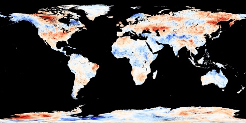
Image from NASA Earth Observations (NEO) for the May 1 to May 31 2012 surface temperature anomalies

Earlier this week, I posted

Comments On Missing Context Information In NOAA’s Report On The Large Positive Land Surface Temperature Anomalies in May 2012

and pointed out a number of problems with the NOAA NCDC data analysis based on the GHCN data, including its warm bias.  Today, I present at the top of this post the May 2012 surface temperature anomaly analysis from NASA’s Earth Observations program.

As written on the NASA’s Earth Observations program website

Land surface temperature is how hot or cold the ground feels to the touch. An anomaly is when something is different from average. These maps show where Earth’s surface was warmer or cooler in the daytime than the average temperatures for the same week or month from 2001-2010. So, a land surface temperature anomaly map for May 2002 shows how that month’s average temperature was different from the average temperature for all Mays between 2001 and 2010.

These maps show land surface temperature anomalies for a given day, week, or month compared to the average conditions during that period between 2000-2008. Places that are warmer than average are red, places that were near-normal are white, and places that are cooler than average are blue. Black means there is no data.

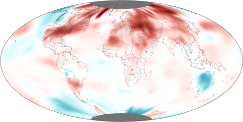
As a reminder, below is the NOAA NCDC analysis for May 2012

It does not take a quantitative analysis to see regions of large differences, such as the cool anomalies in the NASA data in Africa, Scandinavia, and elsewhere. While they are not measuring the same temperatures, the anomalies should be quite similar [For the GHCN, NOAA NCDC uses air temperature measurements which are supposed to be 2m above the ground; they also use the mean temperature anomalies which are computed using maximum and minimum temperatures].

The areal coverage of the temperature anomalies, however, are not the same. The NOAA analysis shows much larger areas of warmer than average surface temperatures than seen in the NASA NEO analysis.

This is yet another documentation of the warm bias in the NOAA NCDC analyses which they use for their press releases on how warm the climate has become. Now that the American Meteorological Society has published its statement “Freedom of Scientific Expression” where they wrote

it is incumbent upon scientists to  communicate their findings in ways that portray their results and the results  of others, objectively, professionally, and without sensationalizing or  politicizing the associated impacts

lets see if Tom Karl, Tom Peterson and others at NCDC finally start to present the diversity of information (and the uncertainties) of what the surface temperature anomalies actually are telling us.

Perspective On The Hot and Dry Continental USA For 2012 Based On The Research Of Judy Curry and Of McCabe Et Al 2004

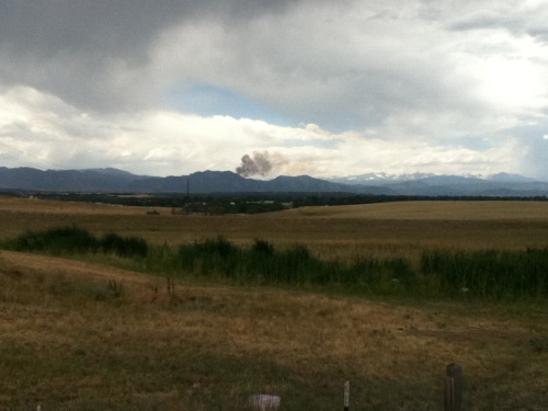
Photo is from June 26 2012 showing start of the June 26 Flagstaff fire near Boulder Colorado

I was alerted to an excellent presentation by Judy Curry [h/t to Don Bishop] which provides an informative explanation of the current hot and dry weather in the USA. The presentation is titled

Climate Dimensions of the Water Cycle by Judy Curry

First, there is an insightful statement by Judy where she writes in slide 5

CMIP century scale simulations are designed for assessing sensitivity to greenhouse gases using emissions scenarios They are not fit for the purpose of inferring decadal scale or regional climate variability, or assessing variations associated with natural forcing and internal variability. Downscaling does not help.

We need a much broader range of scenarios for regions (historical data, simple models, statistical models, paleoclimate analyses, etc). Permit creatively constructed scenarios as long as they can’t be falsified as incompatible with background knowledge.

With respect to the current hot and dry weather, the paper referenced by Judy in her Powerpoint talk

Gregory J. McCabe, Michael A. Palecki, and Julio L. Betancourt, 2004: Pacific and Atlantic Ocean influences on multidecadal drought frequency in the United States. PNAS 2004 101 (12) 4136-4141; published ahead of print March 11, 2004, doi:10.1073/pnas.0306738101

has the abstract [highlight added]

More than half (52%) of the spatial and temporal variance in multidecadal drought frequency over the conterminous United States is attributable to the Pacific Decadal Oscillation (PDO) and the Atlantic Multidecadal Oscillation (AMO). An additional 22% of the variance in drought frequency is related to a complex spatial pattern of positive and negative trends in drought occurrence possibly related to increasing Northern Hemisphere temperatures or some other unidirectional climate trend. Recent droughts with broad impacts over the conterminous U.S. (1996, 1999–2002) were associated with North Atlantic warming (positive AMO) and northeastern and tropical Pacific cooling (negative PDO). Much of the long-term predictability of drought frequency may reside in the multidecadal behavior of the North Atlantic Ocean. Should the current positive AMO (warm North Atlantic) conditions persist into the upcoming decade, we suggest two possible drought scenarios that resemble the continental-scale patterns of the 1930s (positive PDO) and 1950s (negative PDO) drought.

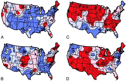
They also present the figure below with the title “Impact of AMO, PDO on 20-yr drought frequency (1900-1999)”.   The figures correspond to A: Warm PDO, cool AMO; B: Cool PDO, cool AMO; C: Warm PDO, warm AMO and D:  Cool PDO, warm AMO

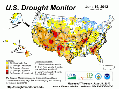
The current Drought Monitor analysis shows a remarkable agreement with D, as shown below

As Judy shows in her talk (slide 8) since 1995 we have been in a warm phase of the AMO and have entered a cool phase of the PDO. This corresponds to D in the above figure.  Thus the current drought and heat is not an unprecedented event but part of the variations in atmospheric-ocean circulation features that we have seen in the past.  This reinforces what Judy wrote that

[w]e need a much broader range of scenarios for regions (historical data, simple models, statistical models, paleoclimate analyses

in our assessment of risks to key resources due to climate. Insightful discussions of the importance of these circulation features are also presented, as just a few excellent examples, by Joe Daleo  and Joe Bistardi on ICECAP, by Bob Tisdale at Bob Tisdale – Climate Observations, and in posts on Anthony Watts’s weblog Watts Up With That.

The 2012 American Meteorological Society Statement “Freedom of Scientific Expression”

The American Meteorological Society has pubished its statement “Freedom of Scientific Expression”. It reads [highlight added]

Advances in science and the benefits of  science to policy,  technological progress, and society as a whole depend upon the free exchange of  scientific data and information as well as on open debate.  The ability of scientists to present their  findings to the scientific community, policy makers, the media, and the public  without censorship, intimidation, or political interference is imperative.  With the specific limited exception of  proprietary information or constraints arising from national security,  scientists must be permitted unfettered communication of scientific results.  In return, it is incumbent upon scientists to  communicate their findings in ways that portray their results and the results  of others, objectively, professionally, and without sensationalizing or  politicizing the associated impacts.

These  principles matter most — and at the same time are most vulnerable to violation  — precisely when science has its greatest bearing on society.  Earth sciences and their applications have  growing implications for public health and safety, economic development,  protection of the environment and ecosystems, and national security.  Thus, scientists, policy makers, and their  supporting institutions share a special responsibility at this time for  guarding and promoting the freedom of responsible scientific expression.

[This statement is considered in force until  September 2017 unless superseded by a new statement issued by the AMS Council  before this date.]

This is a refreshing affirmation of the need for scientific objectivity and the absence of political pressure to limit the presentation of the spectrum of viewpoints on climate and other science issue.

I have posted on a number of examples where such pressure was applied. Among them is the treatment of those who question the robustness of the surface temperature data as applied to diagnosis global warming.  In my public statement

Pielke Sr., Roger A., 2005: Public Comment on CCSP Report “Temperature Trends in the Lower Atmosphere: Steps for Understanding and Reconciling Differences“. 88 pp including appendices

I wrote with regards to this assessment

Future assessment Committees need to appoint members with a diversity of views and who do not have a significant conflict of interest with respect to their own work. Such Committees should be chaired by individuals committed to the presentation of a diversity of perspectives and unwilling to engage in strong-arm tactics to enforce a narrow perspective. Any such committee should be charged with summarizing all relevant literature, even if inconvenient, or which presents a view not held by certain members of the Committee.

Only time will tell, of course, if the guidelines of the AMS Statement will be followed, but at least we now have a formal statement from this professional society that this objectivity and openness is required of its members.

source of image

Comments On Missing Context Information In NOAA’s Report On The Large Positive Land Surface Temperature Anomalies in May 2012

The above figure shows a picture of warmer than average land surface temperatures almost everywhere. This image is from the NOAA report

Global land temperature in May 2012 is warmest on record

It is created, as described in the NOAA article, as a

NOAA map by Dan Pisut, based on Global Historical Climatology Network data from the National Climatic Data Center (NCDC). Caption by Susan Osborne, NCDC. Reviewed by Jessica Blunden, NCDC Climate Monitoring Branch.

However, while it certainly shows a very warm period at the surface, there are caveats in this analysis:

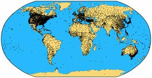
1. The data is not as dense or as uniform as presented in this figure; eg. see the figure below

source of image from climanova.wordpress.com

Large land areas are dependent on just a few or no surface observing sites.

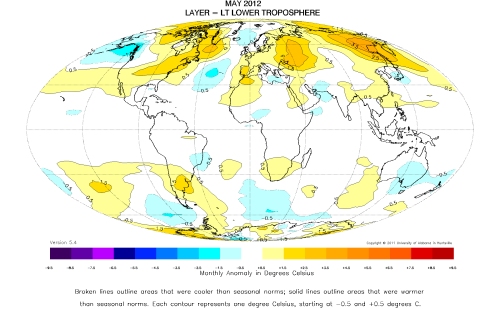
2. While the lower tropospheric data shows a very warm May, it is not as anomalous as at the surface as diagnosed by the Global Historical Climatology Network. The spatial map of lower tropospheric temperatures for May 2012 is shown below

In this data, May 2012 has a global composite lower tropospheric temperature anomaly of +0.29 C (about 0.52 degrees Fahrenheit) above 30-year average for May. The NOAA plot above has a global composite of “more than 1°F above the 20th century average” according to the NOAA article.

3. This divergence between the surface temperature analysis and the lower tropospheric temperature analyses is further demonstration of the divergence between these two data sets as we reported on in

Klotzbach, P.J., R.A. Pielke Sr., R.A. Pielke Jr.,  J.R. Christy, and R.T. McNider, 2009: An alternative explanation for differential temperature trends at the  surface and in the lower troposphere. J. Geophys. Res., 114, D21102, doi:10.1029/2009JD011841.

Klotzbach, P.J., R.A. Pielke Sr., R.A. Pielke Jr.,  J.R. Christy, and R.T. McNider, 2010: Correction to: “An alternative explanation for differential temperature trends at the  surface and in the lower troposphere. J. Geophys. Res., 114, D21102, doi:10.1029/2009JD011841″, J. Geophys. Res.,  115, D1, doi:10.1029/2009JD013655.

In a paper in press, which I will post on soon, we show that there is a warm bias in the minimum land temperatures which are used to create the land temperature anomalies that are presented in the NOAA GHCN figure.

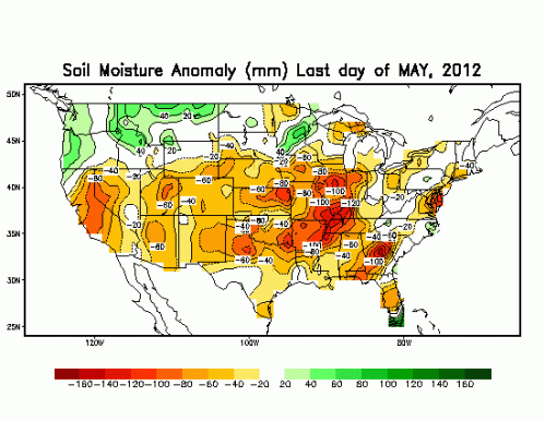
4. The reason that the surface temperature anomaly is so much larger than higher in the troposphere (for the mid tropospheric anomalies, see NOAA CPC) appears to be related to the exceptionally dry soil conditions across much of the USA, as shown for May 2012 below from NOAA’s Climate Prediction Center.

As we discussed in our paper

Pielke, R.A. Sr., K. Wolter, O. Bliss, N. Doesken, and B. McNoldy, 2007:  The July 2005 Denver heat wave: How unusual was it? Nat. Wea. Dig.,  31, 24-35

when the effect of temperature and humidity are combined (moist enthalpy), this provides a markedly different perspective, than using temperature alone. In the July 2005 heat wave discussed in the above paper, the Denver heat wave was less extreme using this combined metric, due to very low humidity accompanying the event. This is also a major factor in the current heat wave.

The mid-tropospheric anomalies for the past 15 days from the University of Albany is presented below which further documents that the tropospheric anomalies over most of the land areas, including the USA, are much less than at the surface.

Thus, the conclusion regarding the NOAA GHCN analysis and the news report based on it is neglects to also report that the same magnitude of anomaly does not exist higher in the troposphere.  Thus the reason for the warm surface temperatures needs further explanation.  In this post I pose that the larger surface temperature anomaly is due to

• the concurrent occurrence of dry soils results in a larger fraction of solar radiation being converted to sensible heat (i.e. measured by the dry bulb temperature) rather than into latent heat fluxes (evaporation and transpiration). This results in a higher dry bulb temperature than it otherwise would be. It is correct, however, that, based on the lower tropospheric temperature analyses, that most land areas appear to be warmer than average for May, but the surface anomalies are significantly larger.
• the surface data also, however, contains an effect of local microclimate changes that results in a local elevation of the nighttime minimum temperatures from what this temperature would have been in the past. The grid-averaging and homogenization algorithms used by NCDC smear this warm effect (which may be applicable only to a very small location) over large areas. This will be discussed further when our new paper is reported on.  This is an issue in addition to the siting quality question in the study led by Anthony Watts that we reported on it Fall et al 2011.
• the use of the GHCN as a diagnostic for the magnitude of global warming has a number of major complications including the neglect of concurrent surface anomalies in water vapor, siting quality issues, and local microclimate effects at GHCN sites which are inappropriately extrapolated over large regions.

Two Papers More Papers On The Important Role Of Regional Circulations on Climate Including Extreme Weather Events

source of image

The importance of regional atmospheric and ocean circulations has been a major theme in my posts on the possible role of humans on the climate system; e.g. see

What is the Importance to Climate of Heterogeneous Spatial Trends in Tropospheric Temperatures?

The most significant effect of human climate forcing  (as well as from natural forcing) is any change in these circulation features over time. A global, annual average surface temperature trend is a useless metric for this purpose.

There is another such regional circulation feature that is the focus of two research papers that has received less scutiny than others such as ENSO, the NAO and the PDO [although colleagues such as Peter Webster and Madhav Khandekar are certainly aware of this climate feature]. This circulation feature is called the Indian Ocean  Dipole (IOD).  The two new papers are

Netrananda Sahu, Swadhin K. Behera, Yosuke Yamashiki, Kaoru Takara and Toshio Yamagata, 2011: IOD and ENSO impacts on the extreme stream-flows of Citarum river in Indonesia, Climate Dynamics 2011, DOI: 10.1007/s00382-011-1158-2

The abstract reads [highlight added]

Extreme stream-flow events of Citarum River are derived from the daily stream-flows at the Nanjung gauge station. Those events are identified based on their persistently extreme flows for 6 or more days during boreal fall when the seasonal mean stream-flow starts peaking-up from the lowest seasonal flows of June–August. Most of the extreme events of high-streamflows were related to La Niña conditions of tropical Pacific. A few of them were also associated with the negative phases of IOD and the newly identified El Niño Modoki. Unlike the cases of extreme high streamflows, extreme low streamflow events are seen to be associated with the positive IODs. Nevertheless, it was also found that the low-stream-flow events related to positive IOD events were also associated with El Nino events except for one independent event of 1977. Because the occurrence season coincides the peak season of IOD, not only the picked extreme events are seen to fall under the IOD seasons but also there exists a statistically significant correlation of 0.51 between the seasonal IOD index and the seasonal streamflows. There also exists a significant lag correlation when IOD of June–August season leads the streamflows of September–November. A significant but lower correlation coefficient (0.39) is also found between the seasonal streamflow and El Niño for September–November season only.

The second paper is

Sahu et al 2012: Large impacts of Indo-Pacific Climate Modes on Extreme Streamflows of Citarum River in Indonesia. J. of Global Environmental Engineering. Vol. 17, pp. 1-8.

The abstract reads [unfortunately, a url does not exist for the paper that I or the author can find].

Large impacts of climate variations modes are found on the extreme stream-flow events of Citarum River derived from the daily stream-flows at the Nanjung gauge station. Extreme events are identified based on their persistent flow for 5 or more days in DJF and MAM seasons when the seasonal mean stream-flows are high. During DJF the positive phases of the Indian Ocean Dipole (IOD) are associated with extremely low-stream-flow events. Except for  one independent IOD events, all low-stream-flow events related to positive IOD events were also associated with El Niño events. However, none of the low-stream-flow events were uniquely associated with El Niño events independent of IOD events in the Indian Ocean. In addition, a few rare low-stream-flow events in DJF associated with La Niña are also accompanied by positive IOD. Therefore, the positive IOD has overwhelmingly negative impacts on stream-flows of Citarum River. The extreme events of high-stream-flows were mostly related to La Niña conditions during DJF  and MAM. Some of the extreme high-flow events were also associated with the negative phases of IOD with a characteristically opposite conditions to that of the positive phase.  Interestingly, La Niña Modokis dominantly influenced the low-stream-flow events when cold anomalies of sea surface temperature flanked the coast of Java-Sumatra in MAM.

Comments On The Paper “Evaluating Explanatory Models Of The Spatial Pattern of Surface Climate Trends Using Model Selection And Bayesian Averaging Methods” By McKitrick and Tole 2012

 

There is a new paper which documents further the lack of skill of multi-decadal climate model predictions. This paper has also been commented on by Judy Curry in the post

Three new papers on interpreting temperature trends

and by Anthony Watts at

New modeling analysis paper by Ross McKitrick.

As I summarized in my post

Kevin Trenberth Was Correct – “We Do Not Have Reliable Or Regional Predictions Of Climate”

these climate model predictions are failing to accurately simulate fundamental aspects of the climate system.

The paper is

McKitrick, Ross R. and Lise Tole (2012) “Evaluating Explanatory Models of the Spatial Pattern of Surface Climate Trends using Model Selection and Bayesian Averaging Methods” Climate Dynamics, 2012, DOI: 10.1007/s00382-012-1418-9

with the abstract [highlight added]

We evaluate three categories of variables for explaining the spatial pattern of warming and cooling trends over land: predictions of general circulation models (GCMs) in response to observed forcings; geographical factors like latitude and pressure; and socioeconomic influences on the land surface and data quality. Spatial autocorrelation (SAC) in the observed trend pattern is removed from the residuals by a well-specified explanatory model. Encompassing tests show that none of the three classes of variables account for the contributions of the other two, though 20 of 22 GCMs individually contribute either no significant explanatory power or yield a trend pattern negatively correlated with observations. Non-nested testing rejects the null hypothesis that socioeconomic variables have no explanatory power. We apply a Bayesian Model Averaging (BMA) method to search over all possible linear combinations of explanatory variables and generate posterior coefficient distributions robust to model selection. These results, confirmed by classical encompassing tests, indicate that the geographical variables plus three of the 22 GCMs and three socioeconomic variables provide all the explanatory power in the data set. We conclude that the most valid model of the spatial pattern of trends in land surface temperature records over 1979-2002 requires a combination of the processes represented in some GCMs and certain socioeconomic measures that capture data quality variations and changes to the land surface.

The text starts off with

General Circulation Models (GCMs) are the basis for modern studies of the effects of greenhouse gases and projections of future global warming. Reliable trend projections at the regional level are essential for policy guidance, yet formal statistical testing of the ability of GCMs to simulate the spatial pattern of climatic trends has been very limited. This paper applies classical regression and Bayesian Model Averaging methods to test this aspect of GCM performance against rival explanatory variables that do not contain any GCM-generated information and can therefore serve as a benchmark.

This paper  supports the viewpoint of the papers

Klotzbach, P.J., R.A. Pielke Sr., R.A. Pielke Jr.,  J.R. Christy, and R.T. McNider, 2009: An alternative explanation for differential temperature trends at the  surface and in the lower troposphere. J. Geophys. Res., 114, D21102, doi:10.1029/2009JD011841.

Klotzbach, P.J., R.A. Pielke Sr., R.A. Pielke Jr.,  J.R. Christy, and R.T. McNider, 2010: Correction to: “An alternative explanation for differential temperature trends at the  surface and in the lower troposphere. J. Geophys. Res., 114, D21102, doi:10.1029/2009JD011841″, J. Geophys. Res.,  115, D1, doi:10.1029/2009JD013655.

where we showed that the multi-decadal trends in surface and lower tropospheric temperature trends are diverging from one another with much greater differences over land areas than over ocean areas. The socioeconomic influences on the land surface and data quality issues identified in the McKittrick and Tole 2012 paper are reasons such a divergence should be expected.

In a paper in press (which I am a co-author on) on the subject of the surface temperature trends, we docuement in depth why there is warm bias in the minumum temperature trends that are used to construct an annual, global average multi-decadal temperture trends. I will be posting on this paper as soon as it is posted on the journal website.  It provides even more support on the findings of McKittrick and Tole 2012 on the importance of socioeconomic influences on the land surface and data quality as a factor in long term temperature trends.

How Well Did The ECMWF Predict The Current Extreme Heat In The Western USA?

In my post on June 14 2012

Hot And Dry Forecast For The Western USA – A Possible Extreme Event

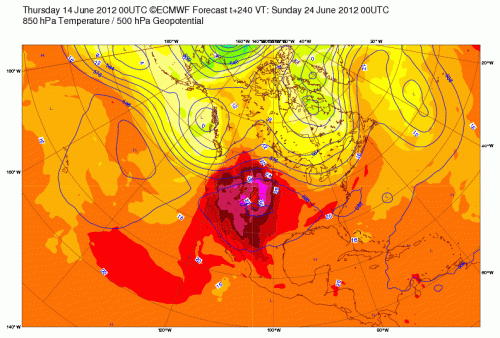
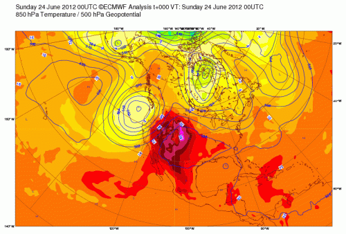
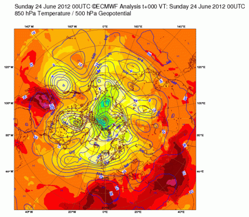
I presented the ECMWF forecast of an extreme heat wave for the western USA. Today’s post is to document how well they did. In my view, it is an outstanding example of how well weather prediction models, which are initialized with real world data, can predict out to 10 days and longer into the future. As just one example of the magnitude of the extreme event, Denver, Colorado matched its all time record June temperature of 104F on June 23.

The ECMWF forecast of 850 hPa temperature and 500 hPa geopotential height made on June 14 2012 00UTC for June 24 2012 00UTC  is reproduced below [click on the image for a clearer view.].

The actual verifying time analysis plots are presented below.

An important conclusion from this heat wave is dominated by regional atmospheric circulation patterns. While the northern hemisphere average positive temperature anomaly could add  to the extreme event, it would be only about +0.44C (+0.8F) [from UAH MSU for May 2012]. Human climate forcings undoubtedly influence atmospheric (and ocean) circulation patterns (e.g. see Pielke et al 2009), such extreme events cannot simply be related directly to “global warming”.

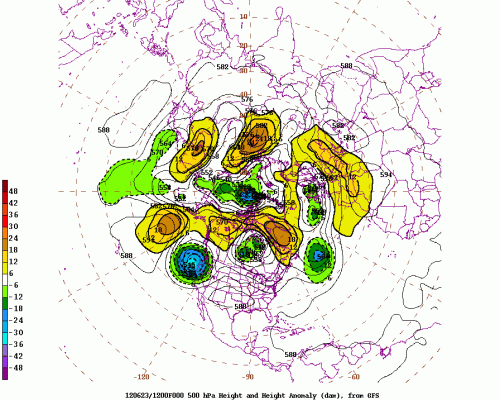
Below is the map of current Northern hemispheric 500 hPa height anomalies which documents the regional characteristic of this extreme event. It also shows that the extreme event was confined to the lower levels of the troposphere, as the 500 hPa anomalies over the western USA are actually dominated by the cold anomaly off of the west coast. It must be the transport north of hot air in the lowest levels of the troposphere from the desert plateau of northern Mexico and the southwest USA which produced the extreme heat (and very dry air) over the Colorado and adjacent areas.

Remarkable Admission By Gavin Schmidt In Response To The McKittrick and Tole 2012 Paper

On Monday, I will have a post on the relationship of the article

McKitrick, Ross R. and Lise Tole (2012) “Evaluating Explanatory Models of the Spatial Pattern of Surface Climate Trends using Model Selection and Bayesian Averaging Methods” Climate Dynamics, 2012, DOI: 10.1007/s00382-012-1418-9

to our research, as his excellent study bolsters our findings.

However, I need to post this afternoon on a remarkable admission by Gavin Schmidt on the McKitrick and Tole paper. In a reply to a comment (#260) by someone who labels themselves as MapleLeaf in the Real Climate post

Unforced Variations; June 2012

Gavin writes [highlight added]

“The basic issue is that for short time scales (in this case 1979-2000), grid point temperature trends are not a strong function of the forcings – rather they are a function of the (unique realisation of) internal variability and are thus strongly stochastic…..There are other issues, but his basic conceptual error is big one from which all other stem”

This is an amazing statement with respect to multi-decadal trends. Perhaps Gavin misspoke. Otherwise, he is stating that that multidecadal local temperature trends are dominated by non-global climate effects and not by the global annual surface temperature tend.  I agree with this view, and am pleased to see recognition of the behavior of the real world climate system from Gavin.

There is also one other remarkable statement as part of this exchange (by MapleLeaf).  MapleLeaf wrote that McKittrick

….also seems to be floating a red herring when he claims that the GCMs are not good at predicting regional changes.  We know that, but what is his point when it comes to reducing GHG emissions?  That we do nothing?”

I actually agree with this view. As my son has written on many times (e.g. see The Climate Fix), the addition of carbon dioxide and other greenhouse gases by human activity to the atmosphere is a first-order climate forcing. The science is settled on this issue. However, where MapleLeaf is missing the point is that huge amounts of research funding and time are being used to apply multi-decadal  regional climate prediction results from the global models (either directly, or dynamically or statistically downscaled)  by the impacts communities; e.g. see.

The Huge Waste Of Research Money In Providing Multi-Decadal Climate Projections For The New IPCC Report

I am pleased to see MapleLeaf also sees this as a waste of money.

I am also glad to see Gavin Schmidt admit to what we have known for a long time –  that a global annual averaged surface temperature trend tells us almost nothing of importance with respect to the risks from climate, including any changes in regional and local climate due to human activities.

source of image

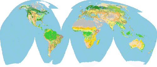
New Paper “Simulating The Biogeochemical And Biogeophysical Impacts Of Transient Land Cover Change And Wood Harvest In The Community Climate System Model (CCSM4) From 1850 to 2100” By Lawrence Et Al 2012

source of image

There is a new global model sensitivity study of the role of land surface processes on the climate system [h/t Rezaul Mahmood]. The new paper is

Lawrence, Peter J., and Coauthors, 2012: Simulating the Biogeochemical and Biogeophysical Impacts of Transient Land Cover Change and Wood Harvest in the Community Climate System Model (CCSM4) from 1850 to 2100. J. Climate, 25, 3071–3095. doi: http://dx.doi.org/10.1175/JCLI-D-11-00256.1

While this paper continues the presentation of time periods in the future (out to 2100) when the CCSM4 has not demonstrated skill at prediction of historical changes in biogeochemical and biogeophysical impacts (i.e. hincast runs), the paper, nevertheless, is an interesting new model sensitivity study. It provides further evidence of the importance of land surface processes within the climate system, as we summarized recently in our paper

Pielke Sr., R.A., A. Pitman, D. Niyogi, R. Mahmood, C. McAlpine, F. Hossain, K. Goldewijk, U. Nair, R. Betts, S. Fall, M. Reichstein, P. Kabat, and N. de Noblet-Ducoudré, 2011: Land  use/land cover changes and climate: Modeling analysis  and  observational evidence. WIREs Clim Change 2011, 2:828–850. doi: 10.1002/wcc.144.

The abstract of the Lawrence et al 2012 paper reads [highlight added]

To assess the climate impacts of historical and projected land cover change in the Community Climate System Model, version 4 (CCSM4), new time series of transient Community Land Model, version 4 (CLM4) plant functional type (PFT) and wood harvest parameters have been developed. The new parameters capture the dynamics of the Coupled Model Intercomparison Project phase 5 (CMIP5) land cover change and wood harvest trajectories for the historical period from 1850 to 2005 and for the four representative concentration pathway (RCP) scenarios from 2006 to 2100. Analysis of the biogeochemical impacts of land cover change in CCSM4 reveals that the model produced a historical cumulative land use flux of 127.7 PgC from 1850 to 2005, which is in general agreement with other global estimates of 156 PgC for the same period. The biogeophysical impacts of the transient land cover change parameters were cooling of the near-surface atmosphere over land by −0.1°C, through increased surface albedo and reduced shortwave radiation absorption. When combined with other transient climate forcings, the higher albedo from land cover change was counteracted by decreasing snow albedo from black carbon deposition and high-latitude warming. The future CCSM4 RCP simulations showed that the CLM4 transient PFT parameters can be used to represent a wide range of land cover change scenarios. In the reforestation scenario of RCP 4.5, CCSM4 simulated a drawdown of 67.3 PgC from the atmosphere into the terrestrial ecosystem and product pools. By contrast the RCP 8.5 scenario with deforestation and high wood harvest resulted in the release of 30.3 PgC currently stored in the ecosystem.

The paper starts with the text

Recent studies have shown that historical human land use and land cover change have significantly impacted the earth’s climate through changes in the carbon cycle, through altered biogeochemical processes (Houghton 2003; Canadell et al. 2007; Bonan 2008; Shevliakova et al. 2009) and through changes in energy and moisture fluxes to the atmosphere, by altering biogeophysical processes (Betts et al. 2001; Feddema et al. 2005; Findell et al. 2007; Bala et al. 2007; Lawrence and Chase 2010).

The evidence that land surface process (both as a climate forcing and as a feedback) are at least as important as other climate forcings, including from the radiative effect of added CO2, are overwhelming, and must be part of an objective assessment of the climate system, as influenced by humans.