A New Paper “Vulnerability To Temperature-Related Hazards: A Meta-Analysis And Meta-Knowledge Approach” By Romero-Lankao Et Al 2012

I was alerted by Professor Karen O’Brien of the University of Oslo to an important new paper that reports on the need to complete textual vulnerabiltiy assessments of risks to key societal and environmental vulnerabilities, as we propose in our article

Pielke Sr., R.A., R. Wilby, D. Niyogi, F. Hossain, K. Dairuku, J. Adegoke, G. Kallos, T. Seastedt, and K. Suding, 2012: Dealing  with complexity and extreme events using a bottom-up, resource-based  vulnerability perspective. AGU Monograph on Complexity and  Extreme Events in Geosciences, in press.

We refer to Karen’s very important research on this topic in our AGU article. In our article we discuss the two approaches to vulnerability:

• the top-down approach (comparitive vulnerability)
• the bottom-up, resource based approach (contextual vulnerability)

The top-down approach (comparitive vulnerability) is the adopted approach in the IPCC reports.

The new paper is

Romero-Lankao, P., et al., 2012: Vulnerability to temperature-related hazards: A meta-analysis and metaknowledge approach. Global Environ. Change.

The abstract reads [highlight added]

Research on urban vulnerability has grown considerably during recent years, yet consists primarily of case studies based on conflicting theories and paradigms. Assessing urban vulnerability is also generally considered to be context-dependent. We argue, however, that it is possible to identify some common patterns of vulnerability across urban centers and research paradigms and these commonalities hold potential for the development of a common set of tools to enhance response capacity within multiple contexts. To test this idea we conduct an analysis of 54 papers on urban vulnerability to temperature- related hazards, covering 222 urban areas in all regions of the world. The originality of this effort is in the combination of a standard metaanalysis with a meta-knowledge approach that allows us not only to integrate and summarize results across many studies, but also to identify trends in the literature and examine differences in methodology, theoretical frameworks and causation narratives and thereby to compare ‘‘apples to oranges.’’ We find that the vast majority of papers examining urban vulnerability to temperature-related hazards come from an urban vulnerability as impact approach, and cities from middle and low income countries are understudied. One of the challenges facing scholarship on urban vulnerability is to supplement the emphasis on disciplinary boxes (e.g., temperature–mortality relationships) with an interdisciplinary and integrated approach to adaptive capacity and structural drivers of differences in vulnerability.

The authors report that “the vast majority of papers examining urban vulnerability to temperature-related hazards come from an urban vulnerability as impact approach“. This is the top-down comparitive vulnerability approach.  The authors argue for a bottom-up (contextual vulnerabilty approach), which Pielke et al 2012 also concluded is needed.

The highlights listed by the authors are:

• Studies on urban vulnerability are based on conflicting theories and paradigms.
• Thirteen factors account for 66% of the tallies of urban vulnerability determinants.
• Reviewed papers mostly come from the urban vulnerability as impact paradigm.
• Scholarship focuses on short time horizons and the city as level of analysis.
• Cities from middle and low-income countries are understudied.

Among the conclusions are

The urban vulnerability as impact lineage is dominatedby epidemiological studies and top-down assessments.

The central message of our study is that what we know depends fundamentally on what questions we ask and how we go about answering those questions (i.e., the kind of methods and data we use or have available to us). Our combined meta-analysis and meta-knowledge exercise highlights the fact that while a great deal of research has been done addressing urban vulnerability to temperature-related hazards, the vast majority of studies fall under a single research paradigm – the urban vulnerability as impacts approach. Although this paradigm has made important contributions to the understanding of urban vulnerability, it tends to ignore other equally fundamental dimensions and determinants; to produce a set of explanatory variables that are tightly constrained by the availability of data, particularly in developing countries; and it omits any attempt to gain ethnographic knowledge of behavioral norms, social networks and risk perceptions that are equally relevant to understanding urban vulnerability.

The dominance of the urban vulnerability as impact paradigm suggests that more studies should be undertaken that apply the inherent urban vulnerability and urban resilience approaches. For instance, studies under an inherent urban vulnerability paradigm can explore underlying societal processes by which assets and options at the individual, family or community level (e.g., self-help housing or access to social networks) allow urban households to adapt, but can also shed light on why in many cases these personal assets are not enough to reduce urban populations’ vulnerability because of the role the state plays in shaping adaptive capacity through such means as promoting economic growth and poverty reduction. Meanwhile, an urban resilience framework holds promise to integrate across disciplines and illuminate a more complete set of drivers of urban vulnerability.

source of image

Comment on the BAMS article “Two Time Scales for The Price Of One (Almost)” By Goddard Et Al 2012

There is an interesting essay in the May issue of BAMS that urges a focus on seasonal and decadal prediction. It is an informative article, but it completely leaves out the issue of where the huge funding of multi-decadal climate prediction fits. The essay is

Goddard, Lisa, James W. Hurrell, Benjamin P. Kirtman, James Murphy, Timothy Stockdale, Carolina Vera, 2012: Two Time Scales for The Price Of One (Almost). Bull. Amer. Meteor. Soc., 93, 621–629.   doi: http://dx.doi.org/10.1175/BAMS-D-11-00220.1

The article starts with the text [highlight added]

While some might call Decadal Prediction the new kid on the block, it would be better to consider it the latest addition to the Climate Prediction family. Decadal Prediction is the fascinating baby that all wish to talk about, with such great expectations for what she might someday accomplish. Her older brother, Seasonal Prediction, is now less talked about by funding agencies and the research community. Given his capabilities, he might seem mature enough to take care of himself, but in reality he is still just an adolescent and has yet to reach his full potential. Much of what he has learned so far, however, can be passed to his baby sister. Decadal could grow up faster than Seasonal did because she has the benefit of her older brother’s experiences. They have similar needs and participate in similar activities, and thus to the extent that they can learn from each other, their maturation is in some ways a mutually reinforcing process. And, while the attention that Decadal brings to the household might seem to distract from Seasonal, the presence of a sibling is actually healthy for Seasonal because it draws attention to the need for and use of climate information, which can bring funding and new research to strengthen the whole Climate Prediction family.

The conclusion reads

The investments described will take considerable human and financial resources and a commitment to sustain them. Compared to the costs of adaptation, the costs of implementing these recommendations will be low, but substantial enough to highlight the need for international coordination to minimize duplication and share the lessons learned throughout the communities involved. These are actions that would be prudent even in the absence of climate change. However, given that climate change has focused global attention on the need for climate information, climate services could build adaptation incrementally through better awareness, preparedness, and resiliency to climate variability at all time scales.

Seasonal and Decadal should not be treated as competitors for the attention of the scientific community. Rather, we should enable them to “play nicely” together, in order to maximize the efforts invested in each.

The essay, however, ignores the subject of multi-decadal climate predictions, and where it fits in this family. One reason for the neglect, of course, is the implicit assumption that such predictions are not contributing signficiantly to the assessment of either seasonal or decadal predictability.

However, I propose the following. If the image of a child and toddler are intended to represent seasonal and decadal prediction, respectively, the image below captures multi-decadal climate prediction. :-)

Grappling With Reality – A Comment On The Skeptical Science Post By Dana1981 “Modeled and Observed Ocean Heat Content – Is There a Discrepancy?”

source of image 

Skeptical Science has a post by dana1981 [where he presents his profile online, but not his name; his photo – sort of – is above – July 24 2012 –  found out from Twitter that is name is Dana Nuccitelli] titled

Modeled and Observed Ocean Heat Content – Is There a Discrepancy?

The short answer is YES. This subject has been discussed in my posts ; e.g. see

Comment On Ocean Heat Content “World Ocean Heat Content And Thermosteric Sea Level Change (0-2000), 1955-2010″ By Levitus Et Al 2012

Jim Hansen’s 1981 Model Prediction Needs Scrutiny

Comments On The Poor Post “Lessons from Past Predictions: Hansen 1981″ By Dana1981 At The Skeptical Science

as well as by Bob Tisdale in his post

Corrections to the RealClimate Presentation of Modeled Global Ocean Heat Content

and in the post by David Evans

The Skeptic’s Case

In the Skeptical Science post by dana1981, he also discusses the issue, and concludes with [highlight added]

In any case, while the OHC issue is not entirely settled in either models or observational data, climate contrarians have exaggerated the possible disrepancy between the two through their standard scientific denial practice of cherrypicking data.  It will be interesting to see how this issue is resolved in the coming years as observational data and climate models improve, and in the forthcoming IPCC Fifth Assessment Report, but in the meantime exaggerating the possible discrepancy is neither constructive nor truly skeptical behavior.

Unfortunately, while he finally (correctly) recognizes that “the OHC issue is not entirely settled in either models or observational data“, he does not seem to recognize his own biases. He has avoided several fundamental issues. His exclusions include:

• There is no need to diagnose a linear trend in upper ocean heat content, if one can accurately measure the heat content in Joules at two different time periods. This difference can be directly used to diagnose the global upper ocean average energy flux over this time period in Watts per meter squared.  The real world ocean itself does the time and space integration.  Thus, using an eyecrometer, all one needs to do is read off the values in Joules at two different time periods.

I discuss this approach in my paper

Pielke Sr., R.A., 2003: Heat storage within the Earth system. Bull. Amer.  Meteor. Soc., 84, 331-335.

Since, there are, of course, uncertainties in the ocean measurements, a range around the best estimates is needed. Levitus et al 2012 did that for their study as did Josh Willis in the figure in my paper

Pielke Sr., R.A., 2008: A broader view of the  role of humans in the climate system. Physics Today, 61, Vol. 11, 54-55.

I suspect the uncertainties in the deeper ocean data of Levitus et al 2012 are too small, given the limited spatial coverage at that depth, but, nonetheless this uncertainty needs to be presented.

The next issue is

• The claim that heat is temporally sequestered in the deeper ocean (a hiatus), avoids the uncomfortable conclusion that this heat is not represented in an global average surface temperature anomaly.

I posted on this, for example, in

Torpedoing Of The Use Of The Global Average Surface Temperature Trend As The Diagnostic For Global Warming

where I wrote that

1.  If heat is being sequestered in the deeper ocean, it must transfer through the upper ocean. In the real world, this has not been seen that I am aware of. In the models, this heat clearly must be transferred  (upwards and downwards) through this layer. The Argo network is spatially dense enough that this should have been see.

2. Even more important is the failure of the authors to recognize that they have devalued the use of the global average surface temperature as the icon to use to communicate the magnitude of global warming.  If this deeper ocean heating actually exists in the real world, it is not observable in the ocean and land surface temperatures. To monitor global warming, we need to keep track of the changes in Joules in the climate system, which, as clearly indicated in the new study by Meehl and colleagues, is not adequately diagnosed by the global, annual-averaged surface temperature trends.

and that

……… if heat really is deposited deep into the ocean (i.e. Joules of heat) it will dispersed through the ocean at these depths and unlikely to be transferred back to the surface on short time periods, but only leak back upwards if at all. The deep ocean would be a long-term damper of global warming, that has not been adequately discussed in the climate science community.

In the paper

Barnett, T.P., D.W. Pierce, and R. Schnur, 2001: Detection of anthropogenic  climate change in the world’s oceans. Science, 292, 270-274

they wrote

“…..a climate model that reproduces the observed change in global air temperature over the last 50 years, but fails to quantitatively reproduce the observed changed in ocean heat content, cannot be correct. The PCM [Parallel Climate Model] has a relatively low sensitivity (less anthropogenic impact on climate) and captures both the ocean- and air-temperature changes. It seems likely that models with higher sensitivity, those predicting the most drastic anthropogenic climate changes in the future, may have difficulty satisfying the ocean constraint.”

The next issue ignored by dana 1981 is that

• The energy flux value of upper ocean heating (when scaled with respect to its estimated fraction of the total magnitude of global warming; e.g. see Hansen’s 2005 estimates here), regardless of the values selected by dana1981 or his commenters from the models and observations, is significantly less than the radiative forcing claimed in the 2007 IPCC report.

As I wrote in my post

Climate Metric Reality Check #1 – The Sum Of Climate Forcings and Feedbacks Is Less Than The 2007 IPCC Best Estimate Of Human Climate Forcing Of Global Warming

If the magnitude of the IPCC estimates of radiative forcings from human causes are greater than or equal to the sum of the total observed radiative forcings and feedbacks (i.e. the total climate system radiative imbalance), then the feedbacks have actually reduced the effect of radiative forcings caused by human activities.  By contrast, if the magnitude of radiative forcing caused by humans is less than the sum of the total observed radiative forcings and feedbacks than the feedbacks have amplified the human radiative forcings.

In this….reality check, the information that is used is

1. Total Radiative Forcing from Human Causes

The radiative forcings from human causes are provided by the 2007 IPCC Report [see page 4 of the Statement for Policymakers; Fig. SPM.2].

Their value is +1.6 [with a range of +0.6 to +2.4 Watts per meter squared]

This value, as reported in a footnote in the IPCC report, is supposed to be a difference with between current and pre-industrial values (but note that that this is not what is stated in the figure caption).

2. Total Observed Radiative Forcings and Feedbacks

Ocean heat content data can be used to diagnose the actual observed climate forcings and feedbacks [Pielke Sr., R.A., 2003: Heat storage within the Earth system]. Here I will use Jim Hansen’s value for the end of the 1990s of

+0.85 Watts per meter squared

(even though this is probably an overstatement (see)).

Thus, the total observed radiative forcing and feedback of 0.85 W/m^2 lies below the IPCC central estimate of 1.6 W/m^2 for just the human contribution to radiative forcing.  This suggests that the climate feedbacks most likely act to diminish the effects of human contributions to radiative forcing, though it is important to recognize that a small part of the IPCC range (0.6 to 0.85) falls under the observed value from the work of Hansen.

This suggests that, at least up to the present, the effect of human climate forcings on global warming has been more muted than predicted by the global climate models.

This issue was inadequately discussed by the 2007 IPCC report. Climate Science has weblogged on this in the past (e.g. see), but so far this rather obvious issue has been ignored.

Dana1981 inadequately examines this issue. Negative forcing from aerosols could explain an observed lower heating, but this would then indicate the 2007 IPCC SPM WG1 estimate of total radiative forcings has significant errors. However, there is an even more significant concern. Where is the positive radiative feedback from claimed increases in atmospheric water vapor? This is an issue ignored in dana1981’s post.

Finally, it is interesting to read the comments which seek to argue that the issues raised in the posts are not very important. For example, one by Tom Curtis reads

So far as I can see, once we use a correct base lining, the divergence issues become the minor issues discussed already by Dana.

At least dana1981 does ask the question –

Modeled and Observed Ocean Heat Content – Is There a Discrepancy?

The answer is YES.

An Interesting Admission And An Error By Gavin Schmidt

Update 28 May 2012 – Gavin’s Responses and My Replies

Gavin responds in OHC Model/Obs Comparison Errata comment #17 by Ken Lambert where he tries (unsuccessfully) to spin that he was talking about the ability to measure the TOA radiative fluxes well enough to close with the upper ocean heat budget changes on annual time periods [I agree on the difficulty of measuring radiative fluxes].  However, within the uncertainty of the upper ocean heat data, it is an accurate measure of what the annual average TOA radiative imbalance is as the ocean itself does the time and space integration.

Gavin wrote originally that

Assuming that there is a direct one-to-one comparison on annual timescales to TOA imbalance is not valid.

I showed he was wrong. He is still in error. He disingenuously writes in his comment that

 “….variations in OHC-700m metric can come from many sources: spatial coverage, ocean internal variability, differences in surface heat flux etc”

Gavin also responds to Ken Lambert’s comment # 18 with

 “There are changes on land, in ice, in the Arctic, in the deep ocean, in the water storage etc. that on a year to year basis are significant.”

Ocean internal variability does not matter except for heat that would be transferred deeper than 700m. Surface heat fluxes are accounted for in the heating of the ocean, as the troposphere has not changed its global heat content in a number of years (e.g. see).  In terms of spatial coverage, such a limitation of coverage is not reported by the Argo research team. Indeed, if that were a problem, I am sure they would be requesting more profilers.  ;-)

The land and sea ice are very small components of the heat within the climate system, as even his colleague Jim Hansen agrees with.  Gavin’s comment about the Arctic makes no sense. Finally, heat transfer to deeper in the ocean should be seen in the Argo network, as has been discussed previously on my weblog. In any case, how much heat does he conclude can be transferred to that depth in any one year?

Gavin finally states that

Our model suggests that OHC-700m is strongly correlated (not perfectly) to the TOA imbalance and is ~90% of the total heat content change.

If he really wanted a scientifically constructive debate, he would present the magnitude of the terms in heat budget outside of the upper ocean. He does agree, in the above statement, that ~90%  of the OHC is in the upper 700m of the ocean. Thus at the very end of his comment, he admits that

There is a direct one-to-one comparison on annual timescales to TOA imbalance.

Gavin, instead of admitting he was wrong (as we are all some of the time), just persists in his erroneous statement instead of modifying it.

On the other issue that Gavin commented on (#20), he writes

Just FWIW, RP Sr’s post today is wrong on both counts. The trend in the historical runs (1951-1999) was 0.15 x 10^22 J/yr, not the trend in the control runs.

However, Gavin wrote in the original post that

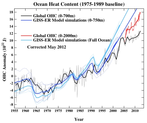
Not sure what is going there. Possibly it could be an issue with control drift. I did a quick analysis of the 1951-1999 trend in the GISS-ER ensemble mean total OHC and it is 0.15 x 10^22 J/yr.

I interpreted the above sentence to mean that the “control drift” was “0.15 x 10^22 J/yr”.  That seemed to be what he is referring to with the use of “it”. If his writing was just sloppy, what is the magnitude of the “control drift” in the GISS runs for the upper ocean heat content in Joules per decade?

I am glad that Gavin has presented his feedback to the insightful comments by Ken Lambert, as this is further documenting the limitation in the quantitative skill of the GISS model to predict global climate system heat changes.

******************************ORIGINAL POST**********************

In Gavin Schmidt’s post

OHC Model/Obs Comparison Errata

he presents an interesting admission and an erroneous statement. First his admission

1. In a reply to the comment by Paul S on Figure 1 in Cai et al. 2010  [#15] on his post

Gavin writes

[Response: Not sure what is going there. Possibly it could be an issue with control drift. I did a quick analysis of the 1951-1999 trend in the GISS-ER ensemble mean total OHC and it is 0.15 x 10^22 J/yr. (0.07 to 0.23  x 10^22 J/yr range within the ensemble). It’s possible that Cai et al is only showing a single run? – gavin]

This documents a linear bias in the GISS multi-decadal model runs of 1.5 x 10^22 J per decade (0.7 to 2.3 x10^22 J per decade).

2. In response to an excellent  comment by Ken Lambert [#17], Gavin writes

Assuming that there is a direct one-to-one comparison on annual timescales to TOA imbalance is not valid.

Gavin is in error as shown in the paper

Ellis et al. 1978: The annual variation in the global heat balance of the Earth. J. Geophys. Res., 83, 1958-1962

and as I have discussed in my paper

Pielke Sr., R.A., 2003: Heat storage within the Earth system. Bull. Amer.  Meteor. Soc., 84, 331-335.

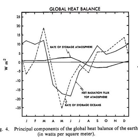
There is a direct relationship between ocean heat content changes and TOA radiative imbalances even on the annual time scale.

I have reproduced below the figure from that paper that shows a direct relationship between the TOA radiative imbalance and ocean heat content is valid. I posted on this recently in

A Summary Of Why The Global Annual-Average Surface Temperature Is A Poor Metric To Diagnose Global Warming

Ken Lambert in his next comment [#18] succinctly also refutes Gavin when he writes

How else is the TOA energy imbalance globally stored in the Earth system if not on the one to one time scale at which it occurs?

It appears that Gavin incompletely appreciates the value of the upper ocean heat storage as a metric to diagnose the magnitude of global warming.  

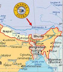
New Paper “Strong Radiative Heating Due To Wintertime Black Carbon Aerosols In The Brahmaputra River Valley” By Chakrabarty Et Al 2012

Papers continue to appear which document that the role of humans on the climate system is much more than that from the emissions of CO2.  One new paper [h/t Marc Morano] is

Chakrabarty, R. K., M. A. Garro, E. M. Wilcox, and H. Moosmüller (2012), Strong radiative heating due to wintertime black carbon aerosols in the Brahmaputra River Valley, Geophys. Res. Lett., 39, L09804, doi:10.1029/2012GL051148.

The abstract reads [highlight added]

The Brahmaputra River Valley (BRV) of Southeast Asia recently has been experiencing extreme regional climate change. A week-long study using a micro-Aethalometer was conducted during January–February 2011 to measure black carbon (BC) aerosol mass concentrations in Guwahati (India), the largest city in the BRV region. Daily median values of BC mass concentration were 9–41 μgm−3, with maxima over 50 μgm−3 during evenings and early mornings. Median BC concentrations were higher than in mega cities of India and China, and significantly higher than in urban locations of Europe and USA. The corresponding mean cloud-free aerosol radiative forcing is −63.4 Wm−2 at the surface and +11.1 Wm−2 at the top of the atmosphere with the difference giving the net atmospheric BC solar absorption, which translates to a lower atmospheric heating rate of ∼2 K/d. Potential regional climatic impacts associated with large surface cooling and high lower-atmospheric heating are discussed.

In the conclusion the authors also write that

The shortwave atmospheric absorption translates to a clear-sky lower atmospheric heating rate of ~2 K/d. This large surface cooling accompanied with significant atmospheric heating could qualitatively explain the regional climate change in the BRV region. Such a situation could intensify low-level inversion, which slows down convection and in turn inhibits cloud formation. Additionally, indirect effects associated with BC aerosols such as the cloud ‘burn off ’ effect [Ackerman et al. 2000] could affect the normal precipitation pattern over this region.

This study adds to the aerosol and land use effects on climate in India that we have docummented in our papers led by Dev Niyogi of Purdue University:

Roy, S.S., R. Mahmood, D. Niyogi, M. Lei, S.A. Foster, K.G. Hubbard, E. Douglas, and R.A. Pielke Sr., 2007: Impacts of the agricultural Green Revolution – induced land use changes on air temperatures in India. J. Geophys. Res. – Special Issue, 112, D21108, doi:10.1029/2007JD008834.

Pielke Sr., R.A., D. Dutta S. Niyogi, T.N. Chase, and J.L. Eastman, 2003:  A new perspective on climate change and variability: A focus on India.  Proc. Indian Natn. Sci. Acad., 69, No. 5, 585-602.

Douglas, E.M., D. Niyogi, S. Frolking, J.B. Yeluripati, R. A. Pielke Sr.,  N. Niyogi, C.J. Vörösmarty, and U.C. Mohanty, 2006: Changes  in moisture and energy fluxes due to agricultural land use and irrigation  in the Indian Monsoon Belt. Geophys. Res. Letts, 33, doi:10.1029/2006GL026550.

Niyogi, D., H.-I. Chang, F. Chen, L. Gu, A. Kumar, S. Menon, and R.A.  Pielke Sr., 2007: Potential impacts of aerosol-land-atmosphere interactions  on the Indian monsoonal rainfall characteristics. Natural Hazards, Special  Issue on Monsoons, Invited Contribution, DOI 10.1007/s11069-006-9085-y.

Douglas, E., A. Beltrán-Przekurat, D. Niyogi, R.A. Pielke, Sr.,  and C. J. Vörösmarty, 2009: The impact of agricultural intensification and  irrigation on land-atmosphere interactions and Indian monsoon precipitation – A  mesoscale modeling perspective. Global Planetary Change, 67, 117–128, doi:10.1016/j.gloplacha.2008.12.007

Lei, M., D. Niyogi, C. Kishtawal, R. Pielke Sr., A. Beltrán-Przekurat, T. Nobis, and S. Vaidya, 2008: Effect of explicit urban land surface representation on the simulation of the 26 July 2005 heavy rain event over Mumbai, India. Atmos. Chem. Phys. Discussions, 8, 8773–8816.

Kishtawal, C.M.,  D. Niyogi, M. Tewari, R.A. Pielke Sr.,  and J. Marshall Shepherd, 2009: Urbanization  signature in the observed heavy rainfall climatology over India.  Int. J. Climatol., 10.1002/joc.2044.

It should be clear to everyone that the human input of CO2 into the atmosphere is only one of climate forcings, and, for at least some regions, is not the dominate one.

source of image

Further Discussion With Zhongfeng Xu On The Value Of Dynamic Downscaling For Multi-Decadal Predictions

In the post

Question And Answer On The Value Of Dynamic Downscaling For Multi-Decadal Predictions

two colleagues of mine and I discussed the significance of their new paper

Xu, Zhongfeng and Zong-Liang Yang, 2012: An improved dynamical downscaling method with GCM bias corrections and its validation with 30 years of climate simulations. Journal of Climate 2012 doi: http://dx.doi.org/10.1175/JCLI-D-12-00005.1

This post continues this discussion with  Zong-Liang Yang of the University of Texas in Austin and Zhongfeng Xu of the Institute of Atmospheric Physics of the Chinese Academy of Science.

Following is the comment by Zhongfeng, with my responses embedded.

Dear Roger,

Thank you for your interest to our paper.

In terms of your comments “their results show that they are not adding value to multi-decadal climate projections”. I think the comment is not accurate enough. We did not compare the climate changes simulated by IDD and TDD in the paper.

My Comment:

What you and Liang have very effectively documented are systematic errors in the observationally unconstrained model runs. You did not compare climate change, but you do show that the model results are biased. This bias is an impediment to skillful multi-decadal forecasts as it shows errors in the model physics and dynamics at that level. The elimination of these errors in the unconstrained runs is a necessary condition for skillful multi-decadal global model predictions.

Zhongfeng continues

So it’s too early to make conclusion whether IDD has adding value to climate change simulation.

My Response

To show skill, one has to show that changes in regional climate statistics between your control and your “future” are skillfully predicted. For model predictions in the coming decades, it is not enough to predict the same climate statistics, one must also skillfully predict changes to these statistics. Otherwise, the impact community could just as well use reanalyses.

Zhongfeng continues

 I guess it’s possible that IDD improves climate change projection when the GCM does a good job in producing climate change signals but producing a bad climatological means.

My Response

This cannot be correct. If the climatological means are in error, there are clearly problems in the model physics and dynamics. Also, what evidence do you have that the GCM does a good job in terms of multi-decadal predictions? [please see my post https://pielkeclimatesci.wordpress.com/2012/05/08/kevin-trenberth-is-correct-we-do-not-have-reliable-or-regional-predictions-of-climate/]

Zhongfeng continues

I will pay more attention to the IDD performance in climate change projection in our future study. I will keep you updated if we find some interesting results.

My Response

I look forward to learning more on your study. Thanks!

Zhongfeng continues

BTW: The IDD does significantly improve the projection of climatological mean. It’s still better than TDD which shows larger bias than IDD in projecting climatological means.

My Response

However, the global model multi-decadal predictions still are run with these biases. Even if you use IDD for the interior, the global model still has these errors meaning they have substantive physics and/or dynamic problems.

Zhongfeng’s comment

 Thank you for all your comments. They are very informative and make me thinking more about this dynamical downscaling study.  ^_^

My Reply 

I have also valued the discussion. I will add this as a weblog post follow-up. Your paper is a very important addition to the literature but the bottom line message is, in my view, documentation of why the impacts communities (e.g. for the IPCC assessments) should not be focusing on this methodology as bracketing the future of regional climates.

source of image

Request To Gavin Schmidt To Update Jim Hansen’s Value Of Upper Ocean Heat Storage Rate

source of image

Update May 23 2012:

Gavin has replied to my question to him below.  I have reproduced it here

[Response: There is nothing incorrect about that statement – this was the result reported in Hansen et al (2005) using the GISS-ER model in CMIP3 – and so there is nothing to update. We will be reporting on the new CMIP5 simulations soon. – gavin]

I appreciate the quick answer from Gavin. It further confirms the overprediction of the GISS-ER heat storage rate.

******************Original Post*************

There is a post at Real Climate titled

OHC Model/Obs Comparison Errata

by Gavin Schmidt that corrects the GISS prediction of changes in ocean heat content over time. Gavin is thanked for his honesty and candor. He wrote in response to one of the comments

armando says:

22 May 2012 at 12:11 PM

That must (have) hurt: http://www.realclimate.org/images/ohc11.jpg

[Response: not really. I learnt a long time ago that a) I’m not infallible, and b) that one should never get personally invested in the results of a model. When things work, one should always remain pleasantly surprised, when they don’t there is possibly a reason that can found – which may be interesting. This is why science is fun. – gavin]

I agree with Gavin’s response. It is refreshing to see him acknowledge that none of us avoid making mistakes, but that we learn from them, and move forward.

There is also an informative post on Gavin’s errata by Bob Tisdale [also reposted at WUWT]

Corrections to the RealClimate Presentation of Modeled Global Ocean Heat Content

including a challenge to Grant Foster [Tamino] to correct his posts.

I have requested Gavin to also correct the GISS values of diagnosed heat storage rate in the following comment which I have submitted on Real Climate

Gavin – Please (you or Jim) update Jim’s diagnosed value of observed upper ocean heat storage rate in Watts per meter squared that he presented in this communication – https://pielkeclimatesci.files.wordpress.com/2009/09/1116592hansen.pdf.

He wrote

“Our simulated 1993-2003 heat storage rate was 0.6 W/m2 in the upper 750 m of the ocean. The decadal mean planetary energy imbalance, 0.75 W/m2, includes heat storage in the deeper ocean and energy used to melt ice and warm the air and land. 0.85 W/m2 is the imbalance at the end of the decade.”

Roger

What we should see is a reduced magnitude of warming from what Jim claimed was occurring when he wrote his earlier comment.  I recently have posted on Jim’s predictions; e.g. see

Jim Hansen’s 1981 Model Prediction Needs Scrutiny

where I wrote that

Lets see if Jim, Gavin Schmidt, or other weblogs that communicate his viewpoint, such as Grant Foster at Tamino and Skeptical Science, respond to this observational study that illustrates a substantive disagreement with the climate model prediction of global warming.  So far they have ignored this disparity between the real world and the models.

I am pleased that Gavin has actually responded to this request for further scrutiny.

Comment On The Blackboard Post “A Surprising Validation of USHCN Adjustments”

source of image WUWT

There is a claim of validation of the BEST data at Blackboard in the post

A Surprising Validation of USHCN Adjustments

by Zeke

He starts off his post with the comment

“Its not often that I get to surprise Richard Muller. But at the Berkeley Earth meeting the other week he was flabbergasted by the results of a simple comparison between CONUS Berkeley data and NCDC’s published USHCN data”

However, Zeke has overlooked several fundamental issues with this claim, that has been the basis for discussion in the comment section on blackboard of Zeke’s post. I have presented several of these below on my weblog, as the issues are so significant (and Muller and Zeke have both ignored so  far) that it is worth bringing to everyone’s attention.

The concerns were succinctly summarized in a comment by Kenneth Fritsch (Comment #96099) who wrote

“(1) What would Zeke’s comparison of the BEST to the three majors’ station inventory look like if it had been in (a) terms of station months and normalized for quality (b) using BEST weighting and (c) accounted for adding new stations to areas which already have good spatial coverage by again using the BEST spatial coverage weighting?”

My way to frame these questions, as I commented on at Blackboard in Comment #95943) , is that

Hi Zeke – There are several issues with the Muller (BEST) approach that need to be resolved. These are discussed in my post

https://pielkeclimatesci.wordpress.com/2011/10/20/comment-on-the-article-in-the-economist-on-rich-mullers-data-analysis/

where I reported what I submitted on Climate Etc that

Hi Judy – I encourage you to document how much overlap there is in Muller’s analysis with the locations used by GISS, NCDC and CRU. In our paper   Pielke Sr., R.A., C. Davey, D. Niyogi, S. Fall, J. Steinweg-Woods, K. Hubbard, X. Lin, M. Cai, Y.-K. Lim, H. Li, J. Nielsen-Gammon, K. Gallo, R. Hale, R. Mahmood, S. Foster, R.T. McNider, and P. Blanken, 2007: Unresolved issues with the assessment of multi-decadal global land surface temperature trends. J. Geophys. Res., 112, D24S08, doi:10.1029/2006JD008229.  we reported that   “The raw surface temperature data from which all of the different global surface temperature trend analyses are derived are essentially the same. The best estimate that has been reported is that 90–95% of the raw data in each of the analyses is the same (P. Jones, personal communication, 2003).”

Zeke – Unless, Muller pulls from a significantly different set of raw data, it is no surprise that his trends are the same. I realize they use more sites, but i) what percent of overlap is there between the HCN and BEST sites  in terms of location and ii) what is the fraction of the time the two sets use different sites (i.e. summing up those stations that both use as compared to the total time of separate BEST and HCN sites)?

Also, what is the siting quality of the non HCN sites used by BEST?

Finally, how do the maximum and minimum temperatures compare?

There remain, in my view substantive unanswered questions. If you have answered this questions already, please refer me to them.

Until these issues are resolved, the quality of Zeke’s analysis and his conclusion remains in limbo. Steve Mosher’s Comment #96066) that

“The only metadata that matters to the algorithm is lat/lon.”

is actually quite an indictment of the BEST analysis and conflicts with almost everything we know about metadata requirements.

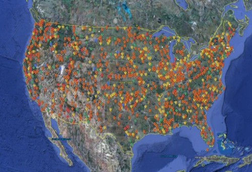
Indeed, Anthony Watts’s seminal research on the quality of the USHCN, exemplified in his first paper on this subject,

Fall, S., A. Watts, J. Nielsen-Gammon, E. Jones, D. Niyogi, J. Christy, and R.A. Pielke Sr., 2011: Analysis of the impacts of station exposure on the U.S. Historical Climatology Network temperatures and temperature trends. J. Geophys. Res.,  116, D14120, doi:10.1029/2010JD015146.Copyright (2011) American Geophysical Union.

illustrates quite convincingly why station metadata, including photographic documentation, is so essential.

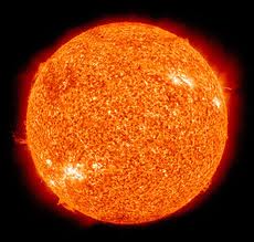
2012 SORCE Science Meeting – Call For Abstracts: “Models Of Spectral Irradiance Variability: Origins In The Solar Atmosphere And Impacts On Earth’s Atmosphere”

2012 SORCE Science Meeting – Call for Abstracts [highlight added]

“Models of Spectral Irradiance Variability: Origins in the solar atmosphere and impacts on Earth’s atmosphere”

September 18-19, 2012  ***   Annapolis, Maryland

http://lasp.colorado.edu/sorce/news/2012ScienceMeeting/index.html

We are pleased to announce the 2012 Solar Radiation and Climate Experiment (SORCE) Science Meeting.  We will examine modeling efforts to understand solar spectral irradiance (SSI) variability, in terms of both its origins in the solar atmosphere and its impact on Earth’s climate and atmosphere. Sessions will be organized around the following key questions:

*         Development of 3-D models of the solar atmosphere are rapidly progressing; how will these models further our understanding of the radiative properties of the solar atmosphere relative to static 1-D models?

*         Do small scale processes on the Sun scale to give irradiance variability, and do they give a reasonable explanation of changes that can occur on decadal or centennial scales that relate to climate change?

*         Does incorporating SSI data into GCMs improve the prediction skills of these models, and do different models produce similar results with the same solar input?

*         For both solar models and GCMs, how well do model predictions agree with observations over decadal time scales?

The format for this meeting consists of invited and contributed presentations in four theme sessions.  We encourage your participation and hope that you will share this announcement with colleagues.  The 2012 Meeting will be held jointly with the NASA GSFC / CU LASP Sun Climate Research Center Symposium.

Deadlines: Abstract:  June 29, 2012 Pre-Registration:  Aug. 17, 2012 Hotel:  Aug. 17, 2012

Thanks, Vanessa George LASP, Univ. of Colorado, Boulder

source of image

My Comment: I am glad that SORCE continues to focus on the Sun-climate relationship and is thinking broadly about the climate issue.

Comments On The Climate Etc Post “CMIP5 Decadal Hindcasts”

Judy Curry has an excellent new paper

Citation: Kim, H.-M., P. J. Webster, and J. A. Curry (2012), Evaluation of short-term climate change prediction in multi-model CMIP5 decadal hindcasts, Geophys. Res. Lett., 39, L10701, doi:10.1029/2012GL051644. [supplemental material]

which she posted on at Climate Etc

CMIP5 decadal hindcasts

I made a suggestion in the comments on her weblog, which I want to also post here on my weblog. First, one of the benchmark which the dynamical model predictions of atmospheric-ocean circulation features must improve on is clearly captured in the seminal paper

Landsea,Christopher W. and ,John A.  Knaff, 2000: How Much Skill Was There in Forecasting the Very Strong 1997–98 El Niño? Bulletin of the American Meteorological Society Volume 81, Issue 9 (September 2000) pp. 2107-2119.

As they wrote

 “A …….simple statistical tool—the El Niño–Southern Oscillation Climatology and Persistence (ENSO–CLIPER) model—is utilized as a baseline for determination of skill in forecasting this event”

and that

“….more complex models may not be doing much more than carrying out a pattern recognition and extrapolation of their own.”

Using persistence which means that the benchmark assumes that the initial values remain constant is not a sufficient test.  Persistance-climatology is the more appropriate evaluation benchmark in which a continuation of a cycle whose future is predicted based on past statistical behavior, given a set of initial conditions. This is what Landsea and Knaff so effectively reported on in their paper for ENSO events. Real world observations, of course, provide the ultimate test of any model prediction, and the reanalysis products, as Kim et al 2012 have done is the best choice.

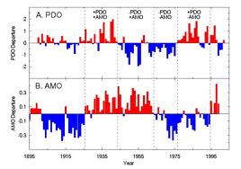
I recommend, therefore,  that Kim et al extend their evaluation to use this benchmark in which the degree to which the CMIP5 decadal predictions can improve on a statistical forecast of the Atlantic Multidecadal Oscillation (AMO) and Pacific Decadal Oscillation (PDO) is examined.

However, it is important to realize, that the CMIP5 runs also need to be tested in terms of their ability to predict changes in the statistical behavior of the AMO and PDO.

Dynamic models need to improve on that skill (i.e. accurately predict changes in this behavior) if those models are going to add any predictive (projection) value in response to human climate forcings. The Kim et al 2012 paper is another valuable, much needed assessment of global model prediction skill. However, the ability of the CMIP5 models to predict changes in the climatological behavior is also needed. Of course, the time period required of observed data is long enough to adequately develop the statistics.

source of image