Geert Jan van Oldenborgh has graciously followed up with me on the posts
with the guest post below. As I wrote in the latter post
The authors should be commended for focusing on this assessment of predictability. We need more such excellent studies!
Decadal prediction skill in a multi-model ensemble
Geert Jan van Oldenborgh, Francisco J. Doblas-Reyes, Bert Wouters, Wilco Hazeleger
Climate predictions are made using climate models, mathematical approximations of the atmosphere, ocean, land surface, snow and ice. The atmospheric part is basically a weather forecast model. The predictability of weather is limited to about two weeks due to the inherent chaos in the atmosphere. However, the climate – statistical properties of the weather – is often predictable on longer time scales. This means that it is impossible to say what the weather will be like on the first of July, but in some regions one can make a skillful forecast that the summer is likely to be warmer than usual. (We disregard the rather trivial forecast that the average temperature in summer is usually higher than in winter.) The main sources of the skill of these seasonal forecasts are El Niño, global warming and persistence. The next step is to make decadal forecasts up to ten years ahead. Theses are fairly new and we would like to know how good these forecasts are. The standard way to investigate this is to run hindcasts: forecasts for the past starting in 1960, 1965, … , 2005 using the current models. Checking these hindcasts against the climate that really occurred gives an idea how good the predictions would have been had the forecast system been available at the time, and by implication how good the forecast for the next ten years is likely to be. In a recently-published article we did just that for four European models, using hindcasts from a EU project (ENSEMBLES).
The main sources of skill of a decadal climate forecast are
- The rising levels of greenhouse gases, mainly CO₂. The CO₂ concentrations has been rising steadily and extrapolating this rise over the next ten years is a safe projection.
- Variations in solar activity and the effects of large tropical volcanic eruptions high in the atmosphere (above 10km). The sunspot cycle is surprisingly hard to predict more than a few years ahead, and the effects of volcanic eruptions only after the eruption itself, so these factors are mostly unknown over most of the forecast.
- The effects of air pollution in the lower part of the atmosphere due to emissions of sulphur, nitrous oxides, sooth and other substances. These can be projected into the future to some extent knowing the sources and the attempts to make these cleaner.
- The predictable part of natural climate variability. To capture this contribution all models were initialized from our best knowledge of the state of the ocean, land, atmosphere and ice.
The four decadal forecast models did not include the effects of volcanic eruptions after the start date, as these would not have been known in a real forecast. We compare the skill of these models with the skill of the CMIP3 ensemble of climate model projections for the previous IPCC report, which do not include initialization. About half of these models include the effects of volcanic eruptions (and usually solar variability), the other half do not.
Global mean temperature
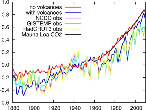
Fig.1 shows three estimates of the observed global mean temperature compared to the CMIP3 projections split into simulations with and without volcanoes. The models that do not include the effect of volcanic eruptions (and most often solar variability) simulate on average a smooth rise of the global mean temperature (red line, natural variability has been much reduced by averaging about 30 different ensemble members.) This rise is described very well by the observed CO₂ concentration scaled to match the modeled global mean temperature (black line). We therefore choose to describe trends as the regression against the CO₂ concentration rather than against time. This also describes the observed temperature trend better, the correlation between the GISTEMP global mean temperature and the observed CO₂ concentration is very good at r=0.91 over 1880-2011, showing that other factors influencing the global mean temperature on long time scales (for instance aerosols) have been proportional to CO₂ concentrations to a large extent.
Figure 1. Global mean 2m temperature anomalies (Jan–Dec annual mean relative to 1931–1960) in the CMIP3 20c3m/sresa1b experiments (with/without volcanoes) compared to the NCDC, GISTEMP and HadCRUT3 SST/T2m reconstructions. The model simulations without volcanic aerosols are compared to observed concentration anomalies scaled by a factor that minimizes the RMS difference between the two series.
The effect of volcanic aerosols can be seen as the large downward peaks in the blue line in Fig. 1 during the years after the eruptions of the Gunung Agung (1963), El Chichón (1982) and Pinatubo (1991). This follows the observations more closely. In the observed global mean temperature the effect of natural variability is also visible. The large El Niño events at the end of 1888, 1914, 1940, 1982 and 1997 caused higher global mean temperatures the next year. Conversely, strong La Niña events caused cooler temperatures than expected on the basis of the trend. Other weather fluctuations, notably winter temperatures in Siberia, also influence the global mean temperature.
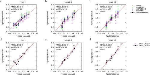
All climate model ensembles we considered have excellent skill in reproducing the observed trend over 1960–2010, see Fig. 2. The ensemble mean trend coincides almost exactly with the observed value, although individual models simulate much higher and lower trends. The CMIP3v sub-ensemble including volcanoes also reproduces some of the variability around the trend. A comparison with the sub-ensemble that does not include volcanoes, CMIP3n, shows that this is mainly due to the inclusion of the effects of volcanic eruptions, However, as this information is not available in a real forecast setting except in the year after an eruption it does not imply real-world skill.
The initialized models also show skill in the first year in predicting variations around the trend of global mean temperature. The runs have been started on Nov. 1, at which time El Niño is well predictable into spring. As the global mean temperature reacts to ENSO with a lag of around five months, this gives some real skill in the annual mean global mean temperature. However, after the first year these models show no skill beyond the trend in forecasting the global mean temperature. A reasonable forecast for the next ten years can therefore be based on a continued rise of CO₂ concentration with 2 ppm/yr times the empirical climate response up to now, 0.085±0.004 K/ppm, giving a 0.17±0.01 K/decade trend, with 2012 likely a bit lower than the trend due to the weak La Niña currently active. Of course this can be upset by a large volcano going off in the tropics. A weak solar cycle could also depress the global mean temperature by 0.03 K or so over the next ten years, successful air pollution controls would increase it somewhat.
Figure 2. Comparison of predicted global mean temperature anomalies (w.r.t.\ 1961–1990) with observed ones (NCDC) of the ENSEMBLES decadal hindcast experiments (a–c) and the CMIP3 ensemble subsets with (CMIP3v) and without (CMIP3n) volcanoes (d–f) for yr 1 (a,d), yrs 2–5 (b,e) and yrs 6–9 (c,f). The red line denotes the best fit to the multi-model (a–c) and CMIP3v (d–f) data, the dashed line the ideal 1:1 agreement. The correlation coefficient, RMSE and regression a (with 1σ error) are given for the multi-model ensemble mean in (a–c) and for the CMIP3v mean in (d–f). The CMIP3n,v ensembles are sampled at the same years as the ENSEMBLES hindcasts.
Local temperature
We next investigate how well the models would have been in forecasting the local temperature if they had been run every five years since 1960. The skill is described by two measures: the correlation coefficient, which shows whether the hindcast and observed temperature series at each grid point varied together, and the regression, which also shows whether the amplitude of the hindcast was correct. For land areas we verify temperature at 2 meters (T2m) against the NCEP GHCN/CAMS dataset, over the oceans we verify sea surface temperature (SST) against ERSST V3b. For the polar regions (south of 60ºS and north of 60ºN) we verify T2m against he GISTEMP 1200 T2m estimate.
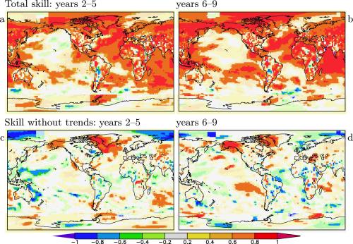
In meteorology, a correlation skill of 0.6 or higher (dark orange or red on the maps) is often considered to be useful, a skill between 0.4 and 0.6 (light orange) may be useful to certain users as a probability forecast, and skills lower than 0.4 (grey, yellow) are usually not useful. Large negative skills implies that opposite forecast would have been skillful. In areas of known model biases this may point to real skill, otherwise they serve as a reminder of the large fluctuations in the skill estimate due to pure chance.
Figure 3. Correlation skill of T2m/SST hindcasts for yrs 2–5 (a,c) and yrs 6–9 (b,d) including the trend (a,b) and the skill that is left after subtracting the local trends (regressions on the CO₂ concentration) of both model and observations (c,d). Correlations that are not significant at p<0.1 are plotted in light colors. SST: ERSST v3b from NCDC, T2m: GHCN/CAMS from NCEP, polar regions: GISTEMP (1200 km decorrelation).
The correlation skill of the four initialized models is shown in Fig. 3a,b. These models show good skill in most areas where there has been a significant trend over this period: most land areas and the Indian and Atlantic Oceans. It should be remembered that the skill estimates are based on 10 or 9 data points only, so they have very large uncertainties. Also, the observational T2m dataset has large uncertainties in areas with few freely available thermometer readings, for instance the noisy areas in South America and Africa where adjoining 2.5º grid boxes have opposite values.
To investigate whether the models have skill beyond the trend we subtracted the best fit to the CO₂ concentration from both the model results and the observations and redid the calculation of the correlation coefficients. The results are shown in Fig. 3c,d. In only a few regions there is clear evidence that the initialized models would have predicted the temperature better than a trend. The most important is the northern North Atlantic Ocean and Labrador Sea, where theory also predicts slowly varying oceanic variability (Atlantic Multidecadal Oscillation, AMO). This is probably connected to the Atlantic Overturning Circulation (AMOC, sometimes also referred to as the “warm Gulf Stream” in popular articles). There may also be predictability beyond the trend in the subtropical Pacific Ocean, where the low-frequency component of ENSO has its expression. This includes the negative skill scores in the West Pacific: in the observations the temperature in these areas varies in opposition to decadal ENSO whereas in the models it has the same sign.
It is tempting to search for skill in areas with known teleconnections to the AMO and decadal ENSO variability. Temperature in the contiguous US and in North Africa and the Middle East is teleconnected to the AMO, in Alaska and the West Pacific there are teleconnections to decadal ENSO. However, over land these teleconnections are so weak (r<0.6) that combined with the imperfect skill in forecasting the AMO (r~0.8 in years 2–5, 0.6 in yrs 6–9) and decadal ENSO (r~0.5 in yrs 2–5, 0.4 in yrs 6–9) themselves the signal becomes undetectable in the small sample of starting dates that we have available. Indeed, there is no skill beyond the trend visible in the US land temperatures except in Alaska. The latter signal is much stronger than expected on the basis of the teleconnection, so we can only ascribe it to a chance fluctuation.
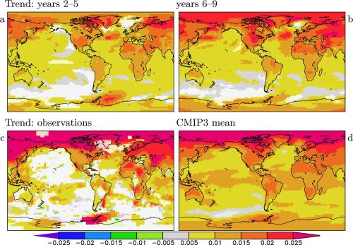
As mentioned before, the correlation coefficient does not tell the whole story. If both the observations and the hindcasts show a trend the correlation coefficient can be high even if the trends are very different. In Fig. 4 we therefore show the trends of the four initialized models and compare these to the trends in the observations and the uninitialized CMIP3 ensemble. Note that trends are again defined as the regression on the CO₂ concentration and therefore have units K/ppm. (The difference with maps of linear trends in K/yr is small.)
Figure 4. The SST/T2m trend [K/ppm] in the ENSEMBLES multi-model ensemble yrs 2–5 (a) and 6–9 (b), for the observations (c) and for the full CMIP3 multi-model mean over 1960–2010 (d, T2m only).
The trends in the initialized models are similar to the trends in the uninitialized CMIP3 ensemble except in the Arctic, where the initialized models severely underestimate the trend. The main features are similar to the observed trends: less warming over the oceans, polar amplification, stronger trends over dry regions. The details are not reproduced very well in either model ensemble: the lack of warming over the North Pacific, southwestern US and adjoining sea, the stronger warming in Europe and Central Asia. We are planning a further publication on the topic whether these discrepancies are within the natural variability. Until the causes are established they are cause for caution in using climate models for local climate forecasts.
Precipitation
Precipitation has much higher variability compared to trends and predictable signals than temperature. The only regions that show skill are northern Europe and the Sahel. In northern Europe a strong trend has been observed in areas where climate models also show a trend, both mainly in winter. As in temperature trends in this region, a problem is that the observed trend is much stronger than the modeled one. In fact both are due to a shift in circulation that may or may not be connected to global warming. Further research is being done to find the causes of the discrepancy in these trends.
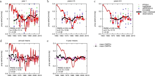
Figure 5. Comparison of predicted Sahel rainfall anomalies [mm/dy] against observed anomalies (GPCC V5 and monitoring analysis) for yr 1 (a), yrs 2–5 (b) and yrs 6–9 (c). Panels (d) and (e) show the same for the CMIP3 ensemble with and without volcanic aerosols. The correlation coefficient, RMSE and regression a (with 1σ error) are given for the ENSEMBLES multi-model ensemble mean in (a–c) and for the CMIP3 models with volcanic aerosols in (d—e).
Sahel rainfall is defined here as the average rainfall over the region 10º–20º N, 18ºW–20ºE. The observations are taken from the GPCC V5 analysis of precipitation. Rainfall in this area is influenced both by the AMO and by decadal ENSO. In the first year, the initialized models have a skill of r=0.5, in years 2–5 the skill is 0.4. The amplitude of the predicted anomalies is however much smaller than the observed variability, with the well-known drought in the 1980s only weakly visible in the hindcasts. Before concluding that the initialization helps in giving some skill in Sahel rainfall forecasts, it should be mentioned that the uninitialized CMIP3v ensemble (including volcanic aerosols) shows similar skill, r=0.5 in 4-yr means but with an even weaker amplitude. A more thorough investigation is needed to find the sources of skill in this area and how they are represented in the climate models. It would be interesting to see whether earlier starting dates reproduce the wet 1950s. Finally, only consultations with end users can show whether this skill, explaining less than 25% of variability in the rainfall averaged over a large area, is useful in practice.
Conclusions
A 4-model 12-member ensemble of 10-yr hindcasts has been analyzed for skill in SST, 2m temperature and precipitation. The main source of skill in temperature is the trend, which is primarily forced by greenhouse gases and aerosols. This trend contributes almost everywhere to the skill. Variation in the global mean temperature around the trend do not have any skill beyond the first year. However, regionally there appears to be skill beyond the trend in the two areas of well-known low-frequency variability: SST in parts of the North Atlantic and Pacific Oceans is predicted better than persistence. A comparison with the CMIP3 ensemble shows that the skill in the northern North Atlantic and eastern Pacific is most likely due to the initialization, whereas the skill in the subtropical North Atlantic and western North Pacific are probably due to the forcing.
There is an indication of skill in hindcasting decadal Sahel rainfall variations, which are known to be teleconnected to North Atlantic and Pacific SST. The uninitialized CMIP3 ensemble that includes volcanic aerosols reproduces these variations as well, but the models without volcanic aerosols do not. It therefore remains an open question whether initialization improves predictions of Sahel rainfall.
The modeled trends agree well with observations in the global mean, but the agreement is not so good at the local scale.
These experiments are only a first step towards decadal forecasting using non-optimized methods from seasonal forecasting. The skill assessment does not take into account the considerable biases and drift of the models. It is based on only nine or ten data points and hence suffers from large statistical uncertainties. Larger ensembles sizes per model and more frequent and earlier starting dates will be required to characterize the skill of decadal forecasts better. The verification of decadal hindcasts can then be used to improve the climate models, their forcings and initialization procedures to give more reliable and skillful climate forecasts.
Journal reference
van Oldenborgh, G.J., F.J. Doblas-Reyes, B. Wouters, W. Hazeleger (2012): Decadal prediction skill in a multi-model ensemble. Clim.Dyn. doi:10.1007/s00382-012-1313-4
A preprint can be downloaded from http://www.knmi.nl/publications/showAbstract.php?id=7603


